untitled
|
|
|
- えりか つまがみ
- 5 years ago
- Views:
Transcription
1 WinLD R (16)
2 WinLD WinLD.zip 2
3 2 1 α = 5% Type I error rate % % % % % 3 Type I error rate = 1 (1α) k
4 Type I error 5% 1 α 5% α 1 α α % % % % % 4
5 1. z-scoreb-value 2. Pocock O'brien-Fleming 3. Lan & DeMets α 4. p 5
6 2 X i i Y i i D i = Y i -X i N( δ, σ 2 ) σ 2 δ = 0 N Z N Z N 1 v N N i 1 D i S v N N, v N var( S N ) N var( D ) 1 n < N n Z { S S S } / v S / v ( S S ) / N n N n N 1n n+1n Z n B-value n N N n v N 6 var
7 2 t v n / v N var( S n ) / var( S N ) 0 1 = 0 = 1 = n/n = ()/() z-scores n /v 1/2 n Z() B-valueB() B ( t ) S n ( ), (1) (1) v N t Z t B Z S v N N 7 trial fractioninformation fraction
8 z-score B-value z-score B-value Z( ),, Z( ) B( ),, B( ) ^ θ = E[Z(1)] = δ / { var(δ) } 1/2... z-score E[Z()] = θ 1/2 cov[z( 1 ), Z( 2 )] = ( 1 / 2 ) 1/2 V[Z()] = 1 B-value E[B()] = θ cov[b( 1 ), B( 2 )] = 1 V[B()] = 8 B() = 1/2 Z()
9 B-value B-value θ B-value ( 1, B(1) ) = ( 1, Z(1) ) (, B() ) B() N( θ, )
10 B-value ^ B() N( θ, ) θ = E[Z(1)] = δ/{ var(δ) } 1/2 B-value ^ ( 1, E[B(1) B(), θ=θ] ) (, B() ) slope = 0 ( 1, E[B(1) B(), θ=0] ) Lan et.al.1988
11 z-score 1.7 = 100/200 = 0.5z-scoreZ(0.5) = 1.7 B-valueB(0.5) = (0.5) 1/2 Z(0.5) = = 1.2 α = Type I error z-score c 1 c 2 Pr{ Z(0.5) > c 1 } = Pr{ Z(0.5) > c 1 or Z(1.0) > c 2 } = c 1 c 2 B-value a 1 a 2 Pr{ B(0.5) > a 1 } = Pr{ B(0.5) > a 1 or B(1.0) > a 2 } = a 1 a 2 11
12 ^ ^ = 100/200 = 0.5δ(0.5) = 0.3se{δ(0.5)} = 0.4 z-scorez(0.5) = 0.3/0.4 = 0.75 B-valueB(0.5) = (0.5) 1/2 Z(0.5) = = 0.53 α = Pr{ Z(0.5) > c 1 } = c 1 c 1 = < seqnorm(0.005, lower=f) = 2.576
13 ^ ^ = 1δ(1.0) = 0.6se{δ(1.0)} = 0.28 ^ z-scorez(1) = 0.6/0.28 = 2.14θ = E[Z(1)] = 2.14 B-valueB(1) = (1) 1/2 Z(1) = 2.14 Type I error Pr{ Z(0.5) > or Z(1.0) > c 2 } = c 2 c 2 = > ^ = var[δ(0.5)] -1 ^ / var[δ(1.0)] -1 ^ = { se[δ(0.5)] } -2 ^ / { se[δ(1.0)] } -2 = 0.5
14 22 Z(1.0) Z(1.0) Z(0.5) Z(0.5) Pr{ Z(1.0) > } Pr{ Z(0.5) 2.576, Z(1.0) > } 14
15 2 15 "Statistical Monitoring of Clinical Trials" findroot()
16 1 = 0.5 Pr{ Z(0.5) > c 1 } = c 1 2 z = z c 1 = = Pr{ Z(0.5) > or Z(1.0) > c 2 } = Pr{ Z(0.5) > } + Pr{ Z(0.5) 2.576, Z(1.0) > c 2 } = Pr{ Z(0.5)2.576, Z(1.0) > c 2 } = 0.02 c 2 2 c 2 = α =
 > c 2 } = 0.02 c 2?")
 } (0, 0 ) ( 1, 1 )")
 c 2 0.")
17 Pr{ Z(0.5)2.576, Z(1.0) > c 2 } = 0.02 c 2?? { Z(0.5)Z(1.0) } (0, 0 ) ( 1, 1 ) (0.5/1.0) 1/2 = c 2 Z(1.0) c c 2 Z(0.5)
18 ^ ^ δ( i ) c i se{δ( i )} c 1 = = ( -0.73, 1.33 ) c 2 = = ( -, 1.20 ) Stagewise ordering 18 repeated confidence interval
19 2 2 2 = n/n = ()/()
20 α c 1 c 2 c 3 Pr{ Z(0.25) > c 1 or Z(0.5) > c 2 or Z(1.0) > c 3 } = c 1 c 2 c Z() B-value B() 50 1 = 0.25Z(0.25) = 1.0B(0.25) = /2 1.0 = = 0.5Z(0.5) = 1.7B(0.2) = 0.5 1/2 1.7 =
21 = 50/180 = = =1 Pr{ Z(0.28) > c 1 or Z(0.56) > c 2 or Z(1.0) > c 3 } = c 1 c (Z( ), Z( ), Z( )) 0 1 ( / ) 1/2 3 (50/200)(100/200) = (50/180)(100/180) = 50/100 Z( ) ( Z( ), Z( )) 21
22 = 50/180 = = =1 c 3 Pr{ Z(0.28) > c 1 or Z(0.56) > c 2 or Z(1.0) > c 3 } = c 3 c 1 c 2 (Z( ), Z( ), Z( )) 0 1 ( / ) 1/2 3 50/200 50/ / /180 ( Z( ), Z( ), Z( )) 22
23 α Pr{ Z(0.25) > c 1 } = c 1 c 1 = α 0.01 Pr{ Z(0.25) > 2.58 or Z(0.5) > c 2 } = 0.01 c 2 c 2 = α Pr{ Z(0.25) > 2.58 or Z(0.5) > 2.49 or Z(1.0) > c 3 } = c 3 c 3 = Pr{ Z(0.28) > 2.58 or Z(0.56) >2.49or Z(1.0) >c 3 } = c 3 c 3 =
24 32 24
25 32 25
26 1. z-scoreb-value 2. Pocock O'brien-Fleming 3. Lan & DeMets α 4. p 26
27 Pocock O'brien-Fleming (Z( ),, Z( )) 0 1 ( / ) 1/2 k Type I error0.025 N N/k Pocock z-score O'brien-Fleming B-value z-score 27
28
29 Pocock k Pr{ 1Z ( i / k ) c ( k )} i α = k=1c(k) = 1.96 k=2c(k) = k=3c(k) = k=4c(k) = k=5c(k) =
30 Pocock k=3
31 Pocock c
32 O'brien-Fleming Pr{ k i 1 B ( i / k ) a( k )} Pr{ k i 1 Z ( i / k ) c ( k )} Pr{ k i 1 Z ( i / k ) a( k ) / t 1 / 2 } α = 0.025k = 5 a(5) = 2.04 Z() = B()/ 1/2 c(1) = 2.04/(1/5) 1/2 = 4.56 c(2) = 2.04/(2/5) 1/2 = 3.23 c(3) = 2.04/(3/5) 1/2 = 2.63 c(4) = 2.04/(4/5) 1/2 = 2.28 c(5) = 2.04/(5/5) 1/2 =
33 O'brien-Fleming k=3k=5
34 O'brien-Fleming c
35 Pocock O'brien-Fleming Pocock 5 O'brien-Fleming 5 35
36 Pocock O'brien-Fleming Pocock z-score O'brien-Fleming B-value z-score 36
37 1. z-scoreb-value 2. Pocock O'brien-Fleming 3. Lan & DeMets α 4. p 37
38 Lan & DeMets α 1 n 2 2n 3 3n Lan & DeMets α α() α(0) = 0 α(1) = α() 38 } ) ( ) ( Pr{ ) ( ) ( ), 1, ( } ) ( Pr{ ) ( j j i i j i j j i i j i j c t Z c t Z t t k j c t Z t
39 Lan & DeMets α Pocock α α p1 () = log{ 1 - (e-1) } Pocock α α p2 () = 0.05 log{ 1 - (e-1) } O'brien-Fleming α α of1 () = 2 { 1 - Φ(z / 1/2 ) } = 2 { 1 - Φ(2.2414/ 1/2 ) } O'brien-Fleming α α of2 () = 4 { 1 - Φ(z / 1/2 ) } = 4 { 1 - Φ(2.2414/ 1/2 ) } Pocock O'brien-Fleming α % 5%
40 Lan & DeMets α 40
41 Lan & DeMets α Pocock z-score O'brien-Fleming B-value 41
42 4α = 0.2, 0.5, 0.8, 1.0 O'brien-Fleming α = c 1 = c 2 = c 3 = 2.266c 4 =
43 43
44 4α 44
45 3 45
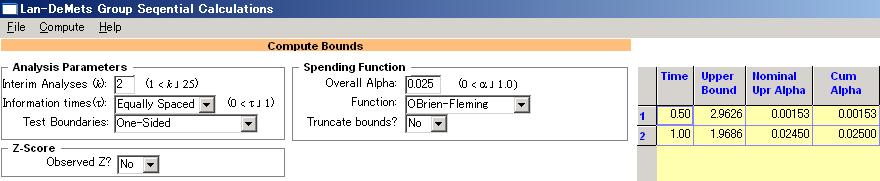
![WinLD Bounds Interim analyses: 4 +[Enter] Info.](/docs-images/91/106755599/images/46-0.jpg "times: User Input Test Bound.: One-Sided Overall Alpha: 0.")
46 WinLD Bounds Interim analyses: 4 +[Enter] Info. times: User Input Test Bound.: One-Sided Overall Alpha: Function: O'brien-Fleming Time Upper Bound
47 α α O'brien-Fleming = 100/200 = α = α = < qt(0.0015, df=200-2, lower=f)
48 52 48
49 α0.025 α α() = = α() = , c 1 = 2.73c 2 = c 1 c 2 c 3 c 3 =
50
51 α0.025 α α() = = 0.5α() = c 1 = = 0.4 = 0.5 α α i ' * ( t ) i { * ( t ) * ( t i )} * ( t i ) 51 α α i α i α α () α
52 = α() = , = = α ' * ( t ) (0.4) t = 0.6 α ' * (0.6) = 0.4,0.6 c 2 = {0.025t (0.4) 1.5 } 52
53 α 53
54 54
55 α Pocock O'brien-Fleming α(0) = 0 α(1) = α() = α() = Z 1, Z 2,... Type I error α 55
56 1. z-scoreb-value 2. Pocock O'brien-Fleming 3. Lan & DeMets α 4. p 56
57 p 9 z???
58 p p p z p 2.5? z p
59 p =0.2z = 2.0 =0.5z = 2.5 (, z ) (, z ) z-score ( 2, z 2 ) ( 1, z 1 ) z-score ordering z-score ( 2, z 2 ) ( 1, z 1 ) z 2 z 1 B-value orderingb-value ( 2, B( 2 ) ) ( 1, B( 1 ) ) 2 1/2 z 2 1 1/2 z 1 MLE ordering Stagewise ordering z-score ( 2, z 2 ) ( 1, z 1 ) 2 1 or 2 = 1 z 2 z 1 59
60 p (, z ) (0.2, 2.0) (0.5, 2.5) 2.2 z-score orderingpr{ (, Z ) (0.5,2.5) } p = Pr{ Z(0.2) 2.2 } + Pr{ Z(0.2) 2.2, Z(0.5) 2.5} + Pr{ Z(0.2) 2.2, Z(0.5) 2.2, Z(1.0) 2.5 } p B-value ordering Pr{ B() 0.5 1/2 2.5) } = Pr{ B() 1.8 } p = Pr{ B(0.2) 1.8 } + Pr{ B(0.2) 1.0, B(0.5) 1.8} + Pr{ B(0.2) 1.0, B(0.5) 1.6, B(1.0) 1.8 } p MLE ordering Stagewise ordering p 60 B() = 1/2 Z()1.0 = 0.2 1/ = 0.5 1/2 2.2
61 Stagewise ordering p j = 2 (, z ) (0.2, 2.0) (0.5, 2.5) 2.2 Stagewise ordering p = Pr{ Z(0.2) 2.2 } p Pr{ Z ( t ) c } Pr{ Z ( t ) j 1 i 1 i i j j + Pr{ Z(0.2) 2.2, Z(0.5) 2.5} = % p z }
 2.")
62 Stagewise ordering p j = 2 (, z ) (0.2, 2.0) (0.5, 2.5) 2.2 Stagewise ordering p = Pr{ Z(0.2) 2.2 } p Pr{ Z ( t ) c } Pr{ Z ( t ) j 1 i 1 i i j j + Pr{ Z(0.2) 2.2, Z(0.5) 2.5} p z } 62
![7p Probability Interim analyses: 5 +[Enter] Info. times: Equally Spaced Test Bound.: One-Sided Upper Bound Determine Bounds: User Input 4 1 = 0.](/docs-images/91/106755599/images/63-0.jpg "2, 2 = 0.4, 3 = 0.6, 4 = 0.8, 5 = 1.0 Upper Bound 4.56, 3.23, 2.63, 2.28, 2.04 O'Brien Fleming 3 z-score 2.94 Stagewise Ordering p 0.001990.")
63 7p Probability Interim analyses: 5 +[Enter] Info. times: Equally Spaced Test Bound.: One-Sided Upper Bound Determine Bounds: User Input 4 1 = 0.2, 2 = 0.4, 3 = 0.6, 4 = 0.8, 5 = 1.0 Upper Bound 4.56, 3.23, 2.63, 2.28, 2.04 O'Brien Fleming 3 z-score 2.94 Stagewise Ordering p % 63
64 X i i Y i i D i = Y i -X i N( δ, σ 2 ) σ 2 ^ ^ ^ ^ 95% ( δ L, δ U ) = ( δ se(δ), δ se(δ) ) ^ z-score z obs Z N( δ L /se(δ), 1 ) δ L Pr{ Z z obs } = α/2 = δ L 64 Pr Z ˆ L se ( ˆ) z obs z PrZ PrZ se ( ˆ) L L se( ˆ) ˆ z z obs ˆ L se ( ˆ) L se ( ˆ) / 2 se ( ˆ) ˆ 1.96 se ( ˆ) 1 / 2 L 1 /2 α = 0.05
65 N(δ,1) z obs δ z α/2 ^ N(δ L /se(δ),1) Pr{Zz obs } = α/2 α/2 ^ δ L /se(δ) z obs 65 95%
66 X i Y i D i = Y i -X i N( δ, σ 2 ) σ 2 ^ ^ ^ 95% ( δ L, δ U ) = ( δ se(δ), δ se(δ) ) ^ z-score z obs Z N(δ U /se(δ), 1 ) δ U Pr{ Z z obs } = δ U ^ δ L /se(δ) z obs ^ δ U /se(δ) 66 95%
67 δ L δ U ^ ^ δ = 3se(δ) = 1z obs = 3 [ -7, 7 ] δ L δ L = -7 Z N( -7, 1 ) Pr{ Z 3 } = 1-Φ(10) = δ L = 0 Z N( 0, 1 ) Pr{ Z 3 } = 1-Φ(3) = δ L = 3.5 Z N( 3.5, 1 ) Pr{ Z 3 } = 1-Φ(-0.5) = δ L = 1.7 Z N( 1.7, 1 ) Pr{ Z 3 } = 1-Φ(1.3) = δ L = 0.8 Z N( 0.8, 1 ) Pr{ Z 3 } = 1-Φ(2.2) = δ L = 1.0 Z N( 1.0, 1 ) Pr{ Z 3 } = 1-Φ(2) = δ L = 1.04 Z N( 1.04, 1 ) Pr{ Z 3 } = 1-Φ(1.96) = δ L = 1.04 δ U = 4.96 δ L δ U ( = grid search) 67 δ L = = 1.04
68 Stagewise ordering Pr{ (, Z ) ( obs,z obs ) } = δ L Pr{ (, Z ) ( obs,z obs ) } = δ U Pr{ (, Z ) ( obs,z obs ) } = 0.5 δ mid ^ θ = δ / se(δ) Pr{ (, Z ) ( obs,z obs ) } = θ L Pr{ (, Z ) ( obs,z obs ) } = θ U Pr{ (, Z ) ( obs,z obs ) } = 0.5 θ mid 68
69 Stagewise ordering Pr{ (, Z ) ( obs,z obs ) } = θ L Pr{ (, Z ) ( obs,z obs ) } = θ U Pr{ (, Z ) ( obs,z obs ) } = 0.5 θ mid z Pr{ Z(0.2) 2.5 } = ^ θ L = δ L /se(δ) Z(0.2) H 0 θ = θ L N( 0.2 1/2 θ L, 1 ) 1 ( = 0.2 ) 2 ( = 0.5 ) 69
70 Stagewise ordering Pr{ (, Z ) ( obs,z obs ) } = θ L Pr{ (, Z ) ( obs,z obs ) } = θ U Pr{ (, Z ) ( obs,z obs ) } = 0.5 θ mid z ( = 0.2 ) ( = 0.5 ) Pr{ Z(0.2) 2.5 } + Pr{ Z(0.2) 2.2, Z(0.5) 2.5 } ^ = θ L = δ L /se(δ) ( Z(0.2), Z(0.5) ) H 0 θ = θ L (0.2 1/2 θ L, 0.5 1/2 θ L ) 1 (0.2/0.5) 1/2 =
71 WinLD Stagewise ordering Pr{ (, Z ) ( obs,z obs ) } = θ L Pr{ (, Z ) ( obs,z obs ) } = θ U Pr{ (, Z ) ( obs,z obs ) } = 0.5 θ mid ^ ^ θ = δ / se(δ) se(δ) 71
72 8 repeated confidence interval 1 = 0.35, 2 = 0.65, 3 = , , z = 2.8 = Pr{ (, Z ) ( obs,z obs ) } = θ L Pr{ Z(0.35) } + Pr{ Z(0.35) , Z(0.65) 2.8} = θ L ( Z(0.35), Z(0.65) ) /2 θ L /2 θ L 1 (0.35/0.65) 1/2 = 0.73 θ L grid-search θ L = 1.0 (0.35 1/2, /2 ) = (0.6, 0.8) Pr{ Z(0.35) } + Pr{ Z(0.35)3.5521, Z(0.65)2.8 } % [ , ] = (0.085, 0.489) =
73 8 73
 1 = 0.35, 2 = 0.65, 3 = 1.02 O'brien-Fleming 3.6128, 2.5503,... 2 z = 2.8 = 0.083 95% [1.03430.083, 5.90160.")
74 8WinLD CI Determine Bounds: Spending Function User Input Standardized Statistics: 2.8 Confidence interval: 0.95 Overall Alpha: 0.05 Function: O'brien-Fleming Time () 1 = 0.35, 2 = 0.65, 3 = 1.02 O'brien-Fleming , ,... 2 z = 2.8 = % [ , ] = (0.085, 0.489) 74

75 9 repeated confidence interval CI Overall Alpha: 0.05 Function: O'brien-Fleming Determine Bounds: Spending Function User Input Standardized Statistics: Confidence interval: 0.95 Time 1 = 0.36, 2 = 0.65, 3 = 1.0 O'brien-Fleming , , z = = % [ , ] = (-0.071, 0.108) 75

76 10Median Unviased Estimator Drift Determine Bounds: User Input Power: () () 1 = 0.15, 2 = 0.25, 3 = 0.4, 4 = 0.7, 5 = , 4.33, 3.36, 2.44, z = = =
77 Stagewise ordering Stagewise ordering p p α 1 p Stagewise ordering p p α θ L > 0 θ U < 0 1 repeated confidence interval Stagewise ordering Stagewise ordering 77 mid-point estimator
78 1. 2. z-scoreb-value 3. Pocock O'brien-Fleming 4. Lan & DeMets α 5. p 78
 1/2 = 3.333 δ = 2, σ = 1.")
79 Probability 1 = 0.17, 2 = 0.33, 3 = 0.50, 4 = 0.67, 5 = 0.83, 6 = , 3.556, 2.903, 2.514, 2.249, = θ = δ/(2σ 2 /18) 1/2 = δ = 2, σ = % 79
80 B() = b B(1) > z α/2 θ z-score E[ B(1) - B() ] = θ(1 - ) V[ B(1) - B() ] = 1 - E θ [ B(1) B()=b ] = b + θ(1 - ) V θ [ B(1) B()=b ] = 1 - CP ( t ) z 1 E [ B (1) B ( t ) / 2 1 t θ b] θ θ = 0 θ ^ = B()/ 80
81 = 0.75B(0.75) = 0.5 slope = E[B()]=3.84E[B(1) B(0.75)=0.5]=1.46 V[B(1) B(0.75)=0.5]=0.25CP 3.84 = 1 - Φ{ ( )/0.25 1/2 } = 1 - Φ(1) = 0.16 ( α=0.05 ) slope = 0 CP 0 = 1 - Φ{ (1.96-0)/0.25 1/2 } 0 ( 1, E[B(1) B(), θ=3.84] ) (, B() ) slope = 0 ( 1, E[B(1) B(), θ=0] ) Lan et.al.1988
82 Statistical Monitoring of Clinical Trials Michael A. Proschan et. al.springer The B-Value: A Tool for Monitoring Data K.K.Grodon Lan et.al.biometrics1988 Multiple Comparisons Using RFrank Bretz et. al.crc press The R Tips 2 R 82
こんにちは由美子です
 Sample size power calculation Sample Size Estimation AZTPIAIDS AIDSAZT AIDSPI AIDSRNA AZTPr (S A ) = π A, PIPr (S B ) = π B AIDS (sampling)(inference) π A, π B π A - π B = 0.20 PI 20 20AZT, PI 10 6 8 HIV-RNA
untitled
 2 : n =1, 2,, 10000 0.5125 0.51 0.5075 0.505 0.5025 0.5 0.4975 0.495 0 2000 4000 6000 8000 10000 2 weak law of large numbers 1. X 1,X 2,,X n 2. µ = E(X i ),i=1, 2,,n 3. σi 2 = V (X i ) σ 2,i=1, 2,,n ɛ>0
AR(1) y t = φy t 1 + ɛ t, ɛ t N(0, σ 2 ) 1. Mean of y t given y t 1, y t 2, E(y t y t 1, y t 2, ) = φy t 1 2. Variance of y t given y t 1, y t
 y t = φy t 1 + ɛ t, ɛ t N(0, σ 2 ) 1. Mean of y t given y t 1, y t 2, E(y t y t 1, y t 2, ) = φy t 1 2. Variance of y t given y t 1, y t") 87 6.1 AR(1) y t = φy t 1 + ɛ t, ɛ t N(0, σ 2 ) 1. Mean of y t given y t 1, y t 2, E(y t y t 1, y t 2, ) = φy t 1 2. Variance of y t given y t 1, y t 2, V(y t y t 1, y t 2, ) = σ 2 3. Thus, y t y t 1,
87 6.1 AR(1) y t = φy t 1 + ɛ t, ɛ t N(0, σ 2 ) 1. Mean of y t given y t 1, y t 2, E(y t y t 1, y t 2, ) = φy t 1 2. Variance of y t given y t 1, y t 2, V(y t y t 1, y t 2, ) = σ 2 3. Thus, y t y t 1,
80 X 1, X 2,, X n ( λ ) λ P(X = x) = f (x; λ) = λx e λ, x = 0, 1, 2, x! l(λ) = n f (x i ; λ) = i=1 i=1 n λ x i e λ i=1 x i! = λ n i=1 x i e nλ n i=1 x
 λ P(X = x) = f (x; λ) = λx e λ, x = 0, 1, 2, x! l(λ) = n f (x i ; λ) = i=1 i=1 n λ x i e λ i=1 x i! = λ n i=1 x i e nλ n i=1 x") 80 X 1, X 2,, X n ( λ ) λ P(X = x) = f (x; λ) = λx e λ, x = 0, 1, 2, x! l(λ) = n f (x i ; λ) = n λ x i e λ x i! = λ n x i e nλ n x i! n n log l(λ) = log(λ) x i nλ log( x i!) log l(λ) λ = 1 λ n x i n =
80 X 1, X 2,, X n ( λ ) λ P(X = x) = f (x; λ) = λx e λ, x = 0, 1, 2, x! l(λ) = n f (x i ; λ) = n λ x i e λ x i! = λ n x i e nλ n x i! n n log l(λ) = log(λ) x i nλ log( x i!) log l(λ) λ = 1 λ n x i n =
k2 ( :35 ) ( k2) (GLM) web web 1 :
 ( k2) (GLM) web web 1 :") 2012 11 01 k2 (2012-10-26 16:35 ) 1 6 2 (2012 11 01 k2) (GLM) kubo@ees.hokudai.ac.jp web http://goo.gl/wijx2 web http://goo.gl/ufq2 1 : 2 2 4 3 7 4 9 5 : 11 5.1................... 13 6 14 6.1......................
2012 11 01 k2 (2012-10-26 16:35 ) 1 6 2 (2012 11 01 k2) (GLM) kubo@ees.hokudai.ac.jp web http://goo.gl/wijx2 web http://goo.gl/ufq2 1 : 2 2 4 3 7 4 9 5 : 11 5.1................... 13 6 14 6.1......................
こんにちは由美子です
 1 2 . sum Variable Obs Mean Std. Dev. Min Max ---------+----------------------------------------------------- var1 13.4923077.3545926.05 1.1 3 3 3 0.71 3 x 3 C 3 = 0.3579 2 1 0.71 2 x 0.29 x 3 C 2 = 0.4386
第11回:線形回帰モデルのOLS推定
 11 OLS 2018 7 13 1 / 45 1. 2. 3. 2 / 45 n 2 ((y 1, x 1 ), (y 2, x 2 ),, (y n, x n )) linear regression model y i = β 0 + β 1 x i + u i, E(u i x i ) = 0, E(u i u j x i ) = 0 (i j), V(u i x i ) = σ 2, i
Mantel-Haenszelの方法
 Mantel-Haenszel 2008 6 12 ) 2008 6 12 1 / 39 Mantel & Haenzel 1959) Mantel N, Haenszel W. Statistical aspects of the analysis of data from retrospective studies of disease. J. Nat. Cancer Inst. 1959; 224):
最小2乗法
 2 2012 4 ( ) 2 2012 4 1 / 42 X Y Y = f (X ; Z) linear regression model X Y slope X 1 Y (X, Y ) 1 (X, Y ) ( ) 2 2012 4 2 / 42 1 β = β = β (4.2) = β 0 + β (4.3) ( ) 2 2012 4 3 / 42 = β 0 + β + (4.4) ( )


1 Stata SEM LightStone 3 2 SEM. 2., 2,. Alan C. Acock, Discovering Structural Equation Modeling Using Stata, Revised Edition, Stata Press.
 1 Stata SEM LightStone 3 2 SEM. 2., 2,. Alan C. Acock, 2013. Discovering Structural Equation Modeling Using Stata, Revised Edition, Stata Press. 2 3 2 Conservative Depress. 3.1 2. SEM. 1. x SEM. Depress.
10:30 12:00 P.G. vs vs vs 2
 1 10:30 12:00 P.G. vs vs vs 2 LOGIT PROBIT TOBIT mean median mode CV 3 4 5 0.5 1000 6 45 7 P(A B) = P(A) + P(B) - P(A B) P(B A)=P(A B)/P(A) P(A B)=P(B A) P(A) P(A B) P(A) P(B A) P(B) P(A B) P(A) P(B) P(B
untitled
 17 5 13 1 2 1.1... 2 1.2... 2 1.3... 3 2 3 2.1... 3 2.2... 5 3 6 3.1... 6 3.2... 7 3.3 t... 7 3.4 BC a... 9 3.5... 10 4 11 1 1 θ n ˆθ. ˆθ, ˆθ, ˆθ.,, ˆθ.,.,,,. 1.1 ˆθ σ 2 = E(ˆθ E ˆθ) 2 b = E(ˆθ θ). Y 1,,Y
報告書
 1 2 3 4 5 6 7 or 8 9 10 11 12 13 14 15 16 17 18 19 20 21 22 2.65 2.45 2.31 2.30 2.29 1.95 1.79 23 24 25 26 27 28 29 30 31 32 33 34 35 36 37 38 39 40 41 42 43 44 45 46 47 60 55 60 75 25 23 6064 65 60 1015
Microsoft Word - 計量研修テキスト_第5版).doc
.doc") Q10-2 テキスト P191 1. 記述統計量 ( 変数 :YY95) 表示変数として 平均 中央値 最大値 最小値 標準偏差 観測値 を選択 A. 都道府県別 Descriptive Statistics for YY95 Categorized by values of PREFNUM Date: 05/11/06 Time: 14:36 Sample: 1990 2002 Included
Q10-2 テキスト P191 1. 記述統計量 ( 変数 :YY95) 表示変数として 平均 中央値 最大値 最小値 標準偏差 観測値 を選択 A. 都道府県別 Descriptive Statistics for YY95 Categorized by values of PREFNUM Date: 05/11/06 Time: 14:36 Sample: 1990 2002 Included
鉄鋼協会プレゼン
 NN :~:, 8 Nov., Adaptive H Control for Linear Slider with Friction Compensation positioning mechanism moving table stand manipulator Point to Point Control [G] Continuous Path Control ground Fig. Positoining
²¾ÁÛ¾õ¶·É¾²ÁË¡¤Î¤¿¤á¤Î¥Ñ¥Ã¥±¡¼¥¸DCchoice ¡Ê»ÃÄêÈÇ¡Ë
 DCchoice ( ) R 2013 2013 11 30 DCchoice package R 2013/11/30 1 / 19 1 (CV) CV 2 DCchoice WTP 3 DCchoice package R 2013/11/30 2 / 19 (Contingent Valuation; CV) WTP CV WTP WTP 1 1989 2 DCchoice package R
1 Stata SEM LightStone 4 SEM 4.. Alan C. Acock, Discovering Structural Equation Modeling Using Stata, Revised Edition, Stata Press 3.
 1 Stata SEM LightStone 4 SEM 4.. Alan C. Acock, 2013. Discovering Structural Equation Modeling Using Stata, Revised Edition, Stata Press 3. 2 4, 2. 1 2 2 Depress Conservative. 3., 3,. SES66 Alien67 Alien71,
nsg02-13/ky045059301600033210
 φ φ φ φ κ κ α α μ μ α α μ χ et al Neurosci. Res. Trpv J Physiol μ μ α α α β in vivo β β β β β β β β in vitro β γ μ δ μδ δ δ α θ α θ α In Biomechanics at Micro- and Nanoscale Levels, Volume I W W v W

1 kawaguchi p.1/81
 1 kawaguchi atsushi@kurume-u.ac.jp 2005 7 2 p.1/81 2.1 2.2 2.2.3 2.3 AUC 4.4 p.2/81 X Z X = α + βz + e α : Z = 0 X ( ) β : Z X ( ) e : 0 σ 2 p.3/81 2.1 Z X 1 0.045 2 0.114 4 0.215 6 0.346 7 0.41 8 0.52
(lm) lm AIC 2 / 1
 lm AIC 2 / 1") W707 s-taiji@is.titech.ac.jp 1 / 1 (lm) lm AIC 2 / 1 : y = β 1 x 1 + β 2 x 2 + + β d x d + β d+1 + ϵ (ϵ N(0, σ 2 )) y R: x R d : β i (i = 1,..., d):, β d+1 : ( ) (d = 1) y = β 1 x 1 + β 2 + ϵ (d > 1) y
W707 s-taiji@is.titech.ac.jp 1 / 1 (lm) lm AIC 2 / 1 : y = β 1 x 1 + β 2 x 2 + + β d x d + β d+1 + ϵ (ϵ N(0, σ 2 )) y R: x R d : β i (i = 1,..., d):, β d+1 : ( ) (d = 1) y = β 1 x 1 + β 2 + ϵ (d > 1) y
数理統計学Iノート
 I ver. 0/Apr/208 * (inferential statistics) *2 A, B *3 5.9 *4 *5 [6] [],.., 7 2004. [2].., 973. [3]. R (Wonderful R )., 9 206. [4]. ( )., 7 99. [5]. ( )., 8 992. [6],.., 989. [7]. - 30., 0 996. [4] [5]
Rによる計量分析:データ解析と可視化 - 第3回 Rの基礎とデータ操作・管理
 R 3 R 2017 Email: gito@eco.u-toyama.ac.jp October 23, 2017 (Toyama/NIHU) R ( 3 ) October 23, 2017 1 / 34 Agenda 1 2 3 4 R 5 RStudio (Toyama/NIHU) R ( 3 ) October 23, 2017 2 / 34 10/30 (Mon.) 12/11 (Mon.)
ECCS. ECCS,. ( 2. Mac Do-file Editor. Mac Do-file Editor Windows Do-file Editor Top Do-file e
 1 1 2015 4 6 1. ECCS. ECCS,. (https://ras.ecc.u-tokyo.ac.jp/guacamole/) 2. Mac Do-file Editor. Mac Do-file Editor Windows Do-file Editor Top Do-file editor, Do View Do-file Editor Execute(do). 3. Mac System
分布
 (normal distribution) 30 2 Skewed graph 1 2 (variance) s 2 = 1/(n-1) (xi x) 2 x = mean, s = variance (variance) (standard deviation) SD = SQR (var) or 8 8 0.3 0.2 0.1 0.0 0 1 2 3 4 5 6 7 8 8 0 1 8 (probability
yamadaiR(cEFA).pdf
.pdf") R 2012/10/05 Kosugi,E.Koji (Yamadai.R) Categorical Factor Analysis by using R 2012/10/05 1 / 9 Why we use... 3 5 Kosugi,E.Koji (Yamadai.R) Categorical Factor Analysis by using R 2012/10/05 2 / 9 FA vs
R 2012/10/05 Kosugi,E.Koji (Yamadai.R) Categorical Factor Analysis by using R 2012/10/05 1 / 9 Why we use... 3 5 Kosugi,E.Koji (Yamadai.R) Categorical Factor Analysis by using R 2012/10/05 2 / 9 FA vs
日本統計学会誌, 第44巻, 第2号, 251頁-270頁
 44, 2, 205 3 25 270 Multiple Comparison Procedures for Checking Differences among Sequence of Normal Means with Ordered Restriction Tsunehisa Imada Lee and Spurrier (995) Lee and Spurrier (995) (204) (2006)
ohpmain.dvi
 fujisawa@ism.ac.jp 1 Contents 1. 2. 3. 4. γ- 2 1. 3 10 5.6, 5.7, 5.4, 5.5, 5.8, 5.5, 5.3, 5.6, 5.4, 5.2. 5.5 5.6 +5.7 +5.4 +5.5 +5.8 +5.5 +5.3 +5.6 +5.4 +5.2 =5.5. 10 outlier 5 5.6, 5.7, 5.4, 5.5, 5.8,
.. F x) = x ft)dt ), fx) : PDF : probbility density function) F x) : CDF : cumultive distribution function F x) x.2 ) T = µ p), T : ) p : x p p = F x
 = x ft)dt ), fx) : PDF : probbility density function) F x) : CDF : cumultive distribution function F x) x.2 ) T = µ p), T : ) p : x p p = F x") 203 7......................................2................................................3.....................................4 L.................................... 2.5.................................
203 7......................................2................................................3.....................................4 L.................................... 2.5.................................
(pdf) (cdf) Matlab χ ( ) F t
 (cdf) Matlab χ ( ) F t") (, ) (univariate) (bivariate) (multi-variate) Matlab Octave Matlab Matlab/Octave --...............3. (pdf) (cdf)...3.4....4.5....4.6....7.7. Matlab...8.7.....9.7.. χ ( )...0.7.3.....7.4. F....7.5. t-...3.8....4.8.....4.8.....5.8.3....6.8.4....8.8.5....8.8.6....8.9....9.9.....9.9.....0.9.3....0.9.4.....9.5.....0....3
(, ) (univariate) (bivariate) (multi-variate) Matlab Octave Matlab Matlab/Octave --...............3. (pdf) (cdf)...3.4....4.5....4.6....7.7. Matlab...8.7.....9.7.. χ ( )...0.7.3.....7.4. F....7.5. t-...3.8....4.8.....4.8.....5.8.3....6.8.4....8.8.5....8.8.6....8.9....9.9.....9.9.....0.9.3....0.9.4.....9.5.....0....3

Stata User Group Meeting in Kyoto / ( / ) Stata User Group Meeting in Kyoto / 21
 Stata User Group Meeting in Kyoto / 21") Stata User Group Meeting in Kyoto / 2017 9 16 ( / ) Stata User Group Meeting in Kyoto 2017 9 16 1 / 21 Rosenbaum and Rubin (1983) logit/probit, ATE = E [Y 1 Y 0 ] ( / ) Stata User Group Meeting in Kyoto
Stata User Group Meeting in Kyoto / 2017 9 16 ( / ) Stata User Group Meeting in Kyoto 2017 9 16 1 / 21 Rosenbaum and Rubin (1983) logit/probit, ATE = E [Y 1 Y 0 ] ( / ) Stata User Group Meeting in Kyoto

A B Z,, Z A Z j ~ N, j B Z ~ N, H 0 : A B H A : A B H 0 : 0, H A : 0 c,, c H 0,, c,, c 0 c 0 H H P P Pr Pr c or c ad c or or c c ad ad c P P c,, c Eat
 A/IML. (998) A/DATA A/IML (998). (998) A B B X A Aj X j,, Bj A: X Aj ~ N, : X Bj ~ N, A B,, ; j,, B Z X A X B Z X A X j X Aj B X Bj j A B Z,, Z A Z j ~ N, j B Z ~ N, H 0 : A B H A : A B H 0 : 0, H A :
N cos s s cos ψ e e e e 3 3 e e 3 e 3 e
 3 3 5 5 5 3 3 7 5 33 5 33 9 5 8 > e > f U f U u u > u ue u e u ue u ue u e u e u u e u u e u N cos s s cos ψ e e e e 3 3 e e 3 e 3 e 3 > A A > A E A f A A f A [ ] f A A e > > A e[ ] > f A E A < < f ; >

y = x x R = 0. 9, R = σ $ = y x w = x y x x w = x y α ε = + β + x x x y α ε = + β + γ x + x x x x' = / x y' = y/ x y' =
 y x = α + β + ε =,, ε V( ε) = E( ε ) = σ α $ $ β w ( 0) σ = w σ σ y α x ε = + β + w w w w ε / w ( w y x α β ) = α$ $ W = yw βwxw $β = W ( W) ( W)( W) w x x w x x y y = = x W y W x y x y xw = y W = w w
chap10.dvi
 . q {y j } I( ( L y j =Δy j = u j = C l ε j l = C(L ε j, {ε j } i.i.d.(,i q ( l= y O p ( {u j } q {C l } A l C l
I L01( Wed) : Time-stamp: Wed 07:38 JST hig e, ( ) L01 I(2017) 1 / 19
 : Time-stamp: Wed 07:38 JST hig e, ( ) L01 I(2017) 1 / 19") I L01(2017-09-20 Wed) : Time-stamp: 2017-09-20 Wed 07:38 JST hig e, http://hig3.net ( ) L01 I(2017) 1 / 19 ? 1? 2? ( ) L01 I(2017) 2 / 19 ?,,.,., 1..,. 1,2,.,.,. ( ) L01 I(2017) 3 / 19 ? I. M (3 ) II,
I L01(2017-09-20 Wed) : Time-stamp: 2017-09-20 Wed 07:38 JST hig e, http://hig3.net ( ) L01 I(2017) 1 / 19 ? 1? 2? ( ) L01 I(2017) 2 / 19 ?,,.,., 1..,. 1,2,.,.,. ( ) L01 I(2017) 3 / 19 ? I. M (3 ) II,
201711grade1ouyou.pdf
 2017 11 26 1 2 52 3 12 13 22 23 32 33 42 3 5 3 4 90 5 6 A 1 2 Web Web 3 4 1 2... 5 6 7 7 44 8 9 1 2 3 1 p p >2 2 A 1 2 0.6 0.4 0.52... (a) 0.6 0.4...... B 1 2 0.8-0.2 0.52..... (b) 0.6 0.52.... 1 A B 2
solutionJIS.dvi
 May 0, 006 6 morimune@econ.kyoto-u.ac.jp /9/005 (7 0/5/006 1 1.1 (a) (b) (c) c + c + + c = nc (x 1 x)+(x x)+ +(x n x) =(x 1 + x + + x n ) nx = nx nx =0 c(x 1 x)+c(x x)+ + c(x n x) =c (x i x) =0 y i (x
meiji_resume_1.PDF
 β β β (q 1,q,..., q n ; p 1, p,..., p n ) H(q 1,q,..., q n ; p 1, p,..., p n ) Hψ = εψ ε k = k +1/ ε k = k(k 1) (x, y, z; p x, p y, p z ) (r; p r ), (θ; p θ ), (ϕ; p ϕ ) ε k = 1/ k p i dq i E total = E
10
 z c j = N 1 N t= j1 [ ( z t z ) ( )] z t j z q 2 1 2 r j /N j=1 1/ N J Q = N(N 2) 1 N j j=1 r j 2 2 χ J B d z t = z t d (1 B) 2 z t = (z t z t 1 ) (z t 1 z t 2 ) (1 B s )z t = z t z t s _ARIMA CONSUME
untitled
 18 1 2,000,000 2,000,000 2007 2 2 2008 3 31 (1) 6 JCOSSAR 2007pp.57-642007.6. LCC (1) (2) 2 10mm 1020 14 12 10 8 6 4 40,50,60 2 0 1998 27.5 1995 1960 40 1) 2) 3) LCC LCC LCC 1 1) Vol.42No.5pp.29-322004.5.
JMP V4 による生存時間分析
 V4 1 SAS 2000.11.18 4 ( ) (Survival Time) 1 (Event) Start of Study Start of Observation Died Died Died Lost End Time Censor Died Died Censor Died Time Start of Study End Start of Observation Censor
.. ( )T p T = p p = T () T x T N P (X < x T ) N = ( T ) N (2) ) N ( P (X x T ) N = T (3) T N P T N P 0
T p T = p p = T () T x T N P (X < x T ) N = ( T ) N (2) ) N ( P (X x T ) N = T (3) T N P T N P 0") 20 5 8..................................................2.....................................3 L.....................................4................................. 2 2. 3 2. (N ).........................................
20 5 8..................................................2.....................................3 L.....................................4................................. 2 2. 3 2. (N ).........................................
?
 240-8501 79-2 Email: nakamoto@ynu.ac.jp 1 3 1.1...................................... 3 1.2?................................. 6 1.3..................................... 8 1.4.......................................
: (EQS) /EQUATIONS V1 = 30*V F1 + E1; V2 = 25*V *F1 + E2; V3 = 16*V *F1 + E3; V4 = 10*V F2 + E4; V5 = 19*V99
 /EQUATIONS V1 = 30*V F1 + E1; V2 = 25*V *F1 + E2; V3 = 16*V *F1 + E3; V4 = 10*V F2 + E4; V5 = 19*V99") 218 6 219 6.11: (EQS) /EQUATIONS V1 = 30*V999 + 1F1 + E1; V2 = 25*V999 +.54*F1 + E2; V3 = 16*V999 + 1.46*F1 + E3; V4 = 10*V999 + 1F2 + E4; V5 = 19*V999 + 1.29*F2 + E5; V6 = 17*V999 + 2.22*F2 + E6; CALIS.
218 6 219 6.11: (EQS) /EQUATIONS V1 = 30*V999 + 1F1 + E1; V2 = 25*V999 +.54*F1 + E2; V3 = 16*V999 + 1.46*F1 + E3; V4 = 10*V999 + 1F2 + E4; V5 = 19*V999 + 1.29*F2 + E5; V6 = 17*V999 + 2.22*F2 + E6; CALIS.
 ( 30 ) 30 4 5 1 4 1.1............................................... 4 1.............................................. 4 1..1.................................. 4 1.......................................
151021slide.dvi
 : Mac I 1 ( 5 Windows (Mac Excel : Excel 2007 9 10 1 4 http://asakura.co.jp/ books/isbn/978-4-254-12172-8/ (1 1 9 1/29 (,,... (,,,... (,,, (3 3/29 (, (F7, Ctrl + i, (Shift +, Shift + Ctrl (, a i (, Enter,
untitled
 146,650 168,577 116,665 122,915 22,420 23,100 7,564 22,562 140,317 166,252 133,581 158,677 186 376 204 257 5,594 6,167 750 775 6,333 2,325 298 88 5,358 756 1,273 1,657 - - 23,905 23,923 1,749 489 1,309
st.dvi
 9 3 5................................... 5............................. 5....................................... 5.................................. 7.........................................................................
all.dvi
 38 5 Cauchy.,,,,., σ.,, 3,,. 5.1 Cauchy (a) (b) (a) (b) 5.1: 5.1. Cauchy 39 F Q Newton F F F Q F Q 5.2: n n ds df n ( 5.1). df n n df(n) df n, t n. t n = df n (5.1) ds 40 5 Cauchy t l n mds df n 5.3: t
% 10%, 35%( 1029 ) p (a) 1 p 95% (b) 1 Std. Err. (c) p 40% 5% (d) p 1: STATA (1). prtesti One-sample test of pr
 p (a) 1 p 95% (b) 1 Std. Err. (c) p 40% 5% (d) p 1: STATA (1). prtesti One-sample test of pr") 1 1. 2014 6 2014 6 10 10% 10%, 35%( 1029 ) p (a) 1 p 95% (b) 1 Std. Err. (c) p 40% 5% (d) p 1: STATA (1). prtesti 1029 0.35 0.40 One-sample test of proportion x: Number of obs = 1029 Variable Mean Std.
1 1. 2014 6 2014 6 10 10% 10%, 35%( 1029 ) p (a) 1 p 95% (b) 1 Std. Err. (c) p 40% 5% (d) p 1: STATA (1). prtesti 1029 0.35 0.40 One-sample test of proportion x: Number of obs = 1029 Variable Mean Std.
こんにちは由美子です
 Analysis of Variance 2 two sample t test analysis of variance (ANOVA) CO 3 3 1 EFV1 µ 1 µ 2 µ 3 H 0 H 0 : µ 1 = µ 2 = µ 3 H A : Group 1 Group 2.. Group k population mean µ 1 µ µ κ SD σ 1 σ σ κ sample mean
.PDF")
<4D6963726F736F667420576F7264202D204850835483938376838B8379815B83578B6594BB2D834A836F815B82D082C88C60202E646F63>
 例 題 で 学 ぶ Excel 統 計 入 門 第 2 版 サンプルページ この 本 の 定 価 判 型 などは, 以 下 の URL からご 覧 いただけます. http://www.morikita.co.jp/books/mid/084302 このサンプルページの 内 容 は, 第 2 版 発 行 当 時 のものです. i 2 9 2 Web 2 Excel Excel Excel 11 Excel
A B P (A B) = P (A)P (B) (3) A B A B P (B A) A B A B P (A B) = P (B A)P (A) (4) P (B A) = P (A B) P (A) (5) P (A B) P (B A) P (A B) A B P
 = P (A)P (B) (3) A B A B P (B A) A B A B P (A B) = P (B A)P (A) (4) P (B A) = P (A B) P (A) (5) P (A B) P (B A) P (A B) A B P") 1 1.1 (population) (sample) (event) (trial) Ω () 1 1 Ω 1.2 P 1. A A P (A) 0 1 0 P (A) 1 (1) 2. P 1 P 0 1 6 1 1 6 0 3. A B P (A B) = P (A) + P (B) (2) A B A B A 1 B 2 A B 1 2 1 2 1 1 2 2 3 1.3 A B P (A
1 1.1 (population) (sample) (event) (trial) Ω () 1 1 Ω 1.2 P 1. A A P (A) 0 1 0 P (A) 1 (1) 2. P 1 P 0 1 6 1 1 6 0 3. A B P (A B) = P (A) + P (B) (2) A B A B A 1 B 2 A B 1 2 1 2 1 1 2 2 3 1.3 A B P (A
DAA12
 Observed Data (Total variance) Predicted Data (prediction variance) Errors in Prediction (error variance) Shoesize 23 24 25 26 27 male female male mean female mean overall mean Shoesize 23 24 25 26 27
Ⅰ.市場リスクの計測手法
 1 2 3 4 { } n n 5 R R R R 1 6 7 8 9 , 10 11 12 13 14 15 T 16 T 17 18 19 20 21 22 23 99VaR 99 24 25 26 0.5 0.5 27 99 28 99 99 29 99 30 31 t-1 t-1 t-1 t-1 t-10 t-10 t-10 t-10 32 33 2 T 2 34 99 99 99 35 36
症例数設定? What is sample size estimation? 医療機器臨床試験のコンサルティングで最も相談件数が多いのは 症例数の設定 Many a need of consulting for device clinical trial is sample size estimat
 医療機器臨床試験における 例数設計のいろは Sample size estimation for clinical trials of devices -First education- 株式会社バイオスタティスティカルリサ - チ古川敏仁 Furukawa Toshihito, Biostatistical Research 2005 年 9 月 3 日第 2 回医療機器臨床試験研究会 Copyright(C)
 ( ) 2002 1 1 1 1.1....................................... 1 1.1.1................................. 1 1.1.2................................. 1 1.1.3................... 3 1.1.4......................................
prime number theorem
 For Tutor MeBio ζ Eite by kamei MeBio 7.8.3 : Bernoulli Bernoulli 4 Bernoulli....................................................................................... 4 Bernoulli............................................................................
Phase II clinical trials for patients with cancer
 II II I 1 I III 14 20 14 20 14 0.05 14 20 1 10 25 20-80 100-200 95 CI (π B π A ) 1.96 [π A (1 π A )/n A + π B (1 π B )/n B ] π A = probability of response rate by treatment A π B = probability of response
自由集会時系列part2web.key
 spurious correlation spurious regression xt=xt-1+n(0,σ^2) yt=yt-1+n(0,σ^2) n=20 type1error(5%)=0.4703 no trend 0 1000 2000 3000 4000 p for r xt=xt-1+n(0,σ^2) random walk random walk variable -5 0 5 variable
R分散分析06.indd
 http://cse.niaes.affrc.go.jp/minaka/r/r-top.html > mm mm TRT DATA 1 DM1 2537 2 DM1 2069 3 DM1 2104 4 DM1 1797 5 DM2 3366 6 DM2 2591 7 DM2 2211 8 DM2

 N N 1,, N 2 N N N N N 1,, N 2 N N N N N 1,, N 2 N N N 8 1 6 3 5 7 4 9 2 1 12 13 8 15 6 3 10 4 9 16 5 14 7 2 11 7 11 23 5 19 3 20 9 12 21 14 22 1 18 10 16 8 15 24 2 25 4 17 6 13 8 1 6 3 5 7 4 9 2 1 12 13

H22 BioS (i) I treat1 II treat2 data d1; input group patno treat1 treat2; cards; ; run; I
 I treat1 II treat2 data d1; input group patno treat1 treat2; cards; ; run; I") H BioS (i) I treat II treat data d; input group patno treat treat; cards; 8 7 4 8 8 5 5 6 ; run; I II sum data d; set d; sum treat + treat; run; sum proc gplot data d; plot sum * group ; symbol c black
H BioS (i) I treat II treat data d; input group patno treat treat; cards; 8 7 4 8 8 5 5 6 ; run; I II sum data d; set d; sum treat + treat; run; sum proc gplot data d; plot sum * group ; symbol c black
1 2 3 1 34060120 1,00040 2,000 1 5 10 50 2014B 305,000140 285 5 6 9 1,838 50 922 78 5025 50 10 1 2
 0120-563-506 / 9001800 9001700 123113 0120-860-777 163-8626 6-13-1 Tel.03-6742-3111 http://www.himawari-life.co.jp 1 2 3 1 34060120 1,00040 2,000 1 5 10 50 2014B 305,000140 285 5 6 9 1,838 50 922 78 5025
k3 ( :07 ) 2 (A) k = 1 (B) k = 7 y x x 1 (k2)?? x y (A) GLM (k
 2 (A) k = 1 (B) k = 7 y x x 1 (k2)?? x y (A) GLM (k") 2012 11 01 k3 (2012-10-24 14:07 ) 1 6 3 (2012 11 01 k3) kubo@ees.hokudai.ac.jp web http://goo.gl/wijx2 web http://goo.gl/ufq2 1 3 2 : 4 3 AIC 6 4 7 5 8 6 : 9 7 11 8 12 8.1 (1)........ 13 8.2 (2) χ 2....................
2012 11 01 k3 (2012-10-24 14:07 ) 1 6 3 (2012 11 01 k3) kubo@ees.hokudai.ac.jp web http://goo.gl/wijx2 web http://goo.gl/ufq2 1 3 2 : 4 3 AIC 6 4 7 5 8 6 : 9 7 11 8 12 8.1 (1)........ 13 8.2 (2) χ 2....................


/はじめに・目次")
P-12 P-13 3 4 28 16 00 17 30 P-14 P-15 P-16 4 14 29 17 00 18 30 P-17 P-18 P-19 P-20 P-21 P-22
 1 14 28 16 00 17 30 P-1 P-2 P-3 P-4 P-5 2 24 29 17 00 18 30 P-6 P-7 P-8 P-9 P-10 P-11 P-12 P-13 3 4 28 16 00 17 30 P-14 P-15 P-16 4 14 29 17 00 18 30 P-17 P-18 P-19 P-20 P-21 P-22 5 24 28 16 00 17 30 P-23


1 Tokyo Daily Rainfall (mm) Days (mm)
 Days (mm)") ( ) r-taka@maritime.kobe-u.ac.jp 1 Tokyo Daily Rainfall (mm) 0 100 200 300 0 10000 20000 30000 40000 50000 Days (mm) 1876 1 1 2013 12 31 Tokyo, 1876 Daily Rainfall (mm) 0 50 100 150 0 100 200 300 Tokyo,
( ) r-taka@maritime.kobe-u.ac.jp 1 Tokyo Daily Rainfall (mm) 0 100 200 300 0 10000 20000 30000 40000 50000 Days (mm) 1876 1 1 2013 12 31 Tokyo, 1876 Daily Rainfall (mm) 0 50 100 150 0 100 200 300 Tokyo,
) ] [ h m x + y + + V x) φ = Eφ 1) z E = i h t 13) x << 1) N n n= = N N + 1) 14) N n n= = N N + 1)N + 1) 6 15) N n 3 n= = 1 4 N N + 1) 16) N n 4
![) ] [ h m x + y + + V x) φ = Eφ 1) z E = i h t 13) x << 1) N n n= = N N + 1) 14) N n n= = N N + 1)N + 1) 6 15) N n 3 n= = 1 4 N N + 1) 16) N n 4](/thumbs/92/107866707.jpg ") ] [ h m x + y + + V x) φ = Eφ 1) z E = i h t 13) x << 1) N n n= = N N + 1) 14) N n n= = N N + 1)N + 1) 6 15) N n 3 n= = 1 4 N N + 1) 16) N n 4") 1. k λ ν ω T v p v g k = π λ ω = πν = π T v p = λν = ω k v g = dω dk 1) ) 3) 4). p = hk = h λ 5) E = hν = hω 6) h = h π 7) h =6.6618 1 34 J sec) hc=197.3 MeV fm = 197.3 kev pm= 197.3 ev nm = 1.97 1 3 ev
1. k λ ν ω T v p v g k = π λ ω = πν = π T v p = λν = ω k v g = dω dk 1) ) 3) 4). p = hk = h λ 5) E = hν = hω 6) h = h π 7) h =6.6618 1 34 J sec) hc=197.3 MeV fm = 197.3 kev pm= 197.3 ev nm = 1.97 1 3 ev
Part () () Γ Part ,
 () Γ Part ,") Contents a 6 6 6 6 6 6 6 7 7. 8.. 8.. 8.3. 8 Part. 9. 9.. 9.. 3. 3.. 3.. 3 4. 5 4.. 5 4.. 9 4.3. 3 Part. 6 5. () 6 5.. () 7 5.. 9 5.3. Γ 3 6. 3 6.. 3 6.. 3 6.3. 33 Part 3. 34 7. 34 7.. 34 7.. 34 8. 35
Contents a 6 6 6 6 6 6 6 7 7. 8.. 8.. 8.3. 8 Part. 9. 9.. 9.. 3. 3.. 3.. 3 4. 5 4.. 5 4.. 9 4.3. 3 Part. 6 5. () 6 5.. () 7 5.. 9 5.3. Γ 3 6. 3 6.. 3 6.. 3 6.3. 33 Part 3. 34 7. 34 7.. 34 7.. 34 8. 35
SFGÇÃÉXÉyÉNÉgÉãå`.pdf
 SFG 1 SFG SFG I SFG (ω) χ SFG (ω). SFG χ χ SFG (ω) = χ NR e iϕ +. ω ω + iγ SFG φ = ±π/, χ φ = ±π 3 χ SFG χ SFG = χ NR + χ (ω ω ) + Γ + χ NR χ (ω ω ) (ω ω ) + Γ cosϕ χ NR χ Γ (ω ω ) + Γ sinϕ. 3 (θ) 180
スライド 1
 SAS による二項比率の差の非劣性検定の正確な方法について 武藤彬正宮島育哉榊原伊織株式会社タクミインフォメーションテクノロジー Eact method of non-inferiority test for two binomial proportions using SAS Akimasa Muto Ikuya Miyajima Iori Sakakibara Takumi Information


