- PDF Free Download

Size: px

Start display at page:

Download ""

ぜんすけにいだ
5 years ago
Views:

1 ( ) 1 1.1?

3 ( ) ( ) ( ) 1.1(a) T m ( ) 1.1(a) T g ( ) T g T g

4 500 74% ( ) T K ( 1.1(b) 15 T g T g T g

5 T g T g [ ] A ( ) exp (1.1) T T 0 Vogel-Fulcher T 0 T 0 T K T K Ortho-Terphenil (OTP) SiO 2 (1.1) T 0 = 0 exp[a/t ] exp [ E/k B T ] 1.2?? T K

6 exp [A/T ] (1.1) [2] [2] [3]

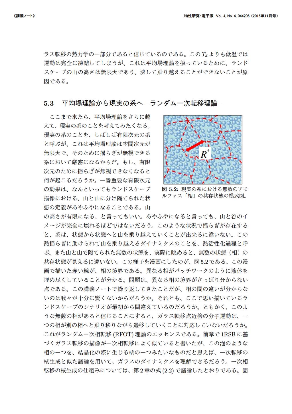
7 ( ) Soft Glassy Materials RNA [4] [5] ( ) [6] ( )

8 [7] [8, 9] ( ) 2 τ exp[a/t ] T = T c

10 E = σr 2 G (2.2) R ( ) σ G = G crystal G liq (Gibbs) G R 3 R R 2 R 3 R 2.1(a) ρ(r) ( S(k) ) S(k) (b) [11] (dynamic heterogeneneities)

11 [11,12] Adam-Gibbs [13] (mode-coupling theory, MCT)

13 T = T = 0 exp[b/t 2 ] 4 (RFOT) (MCT) RFOT MCT (MCT) MCT MCT 1950 [17] MCT

14 MCT [18] 1980 Kirkpatrick MCT MCT [19] MCT ρ m v ρ m = (ρ m v) t ρ m v t + (ρ m vv) = p + η 2 v + (ζ + 13 η ) v (4.1) p η ζ ρ m ρ m v ρ = ρ m /m δρ (4.1) 2 δρ k t 2 = c 2 k 2 δρ k Γk 2 δρ k t (4.2) ρ 0 Γ = (ζ + 4η/3)/ρ m c = 1/ ρ 0 χ χ = V 1 ( V/ p) T δρ k e zt (4.2) z = ± c 2 k 2 + Γ 2 k 4 /4 Γk 2 /2 (4.3)

15 k k 2 z ±ick 1 2 Γk2 k (4.3) k (4.2) δρ k t = c2 k 2 Γk 2 δρ k (4.4) ( k 2 ) Γ Γ(k) Γ(k) k 2 Γk 2 Γk 2 = ζ c c(k) k c(k) χ 12 [10] N 1 N 2 = ρ 0 k B T χ N (2.1) N ρ 0 k B T χ = dr δρ(r)δρ(0) (4.5) 2.1(a) S(k) (4.5) c 2 ρ 0 k B T χ = lim k 0 S(k) (4.6) c 2 k BT S(k) (4.4) (4.7) δρ k t = Dk2 S(k) δρ k (4.8) D = k B T/ζ (4.8) S(k) S(k) 2.1(a)

16 de Genne Narrowing (4.8) (4.8) δρ k t = Dk2 S(k) δρ k D dq k qc(k q)δρ k q δρ q (4.9) c(k) [20] dx dt = µx Vx2 (4.10) C(t) = x(t)x(0) x(0) C(t) = µc(t) + 1 t 2 VC 2,1(t) (4.11) C 2,1 (t) x 2 (t)x(0) 3 x(t) C 2,1 (t) = C 1,2 (t) x(t)x 2 (0) C 1,2 (t) C 1,2 (t) t = µc 1,2 (t) VC 2,2(t) (4.12) C 2,2 (t) = x 2 (t)x 2 (0) 4 (4.12) C 2,1 (t) = t 0 dt e µ(t t ) 1 2 VC 2,2(t ) = t 0 dt 1 2 VC 2,2(t t )C (0) (t ) (4.13) C (0) (t) = e µt 0 C(t) (4.11) C(t) t = µc(t) t 0 dt V 2 C 2,2 (t t )C (0) (t ) (4.14)

19 p = 3 [21] H = N J ijk S i S j S k (5.1) ijk S i (i = 1,, N) J ijk S i N Si 2 = N (5.2) i N 1 i S i q = 1 S i 2 (5.3) N (overlap) J ijk ( ) i F = k B T ln Z (5.4) Z J ijk ln x = lim n 0 x n 1 n (5.5) n n 0 J ijk n q = 0 q q 0 = 0 q 1 ( 0)

21 T K S c S c 1 1.1(a) S c 3 ( [22] 4 ) S i t = µs i H S i + f i (5.6) f i f i (t)f i (t ) = 2k B T δ(t t ) [21] µ (5.2) (5.1) S i t = µs i jk J ijk S j S k + f i (5.7) (4.10) C(t) = N 1 i S i(t)s i (0) dc(t) dt = µc(t) + 3J 2 2k B T t 0 dt C 2 (t t ) dc(t ) dt (5.8) (4.16) 4.1 T d T d

23 (2.2) E = σr θ s c R 3 (5.9) s c S c /N θ E R R = (σ/s c ) 1/(d θ) R E τ exp [ E /T ] E [ ] s c R s θ/(d θ) c τ exp s c T = T K As θ/(d θ) c s c a(t T K ) θ = d/2 [ ] A τ exp T T K (1.1) (5.10) 4 T d ( ) T d ( T K ( ) R

24 6? ( ) ( ) 64% [23]

25 1RSB [24] [1] C. A. Angell, J. Non-Cryst. Solids 102, 205 (1988). [2], (, 2005). [3], ( ). [4] D. Goodsell, [5] R. J. Ellis and A. P. Minton, Nature 425, 27 (2003). [6] T. E. Angelini et al., Proc. Nat. Acad. Sci., 108, 4714 (2011). [7] A. Vespignani, Nature 464, 984 (2010). [8],, 94, 137 (2010). [9] M. Mézard and A. Montanari, Information, Physics, and Computation (Oxford, 2009). [10],, ( ). [11] E. R. Weeks, et. al. Science 287, 627 (2000). [12] R. Yamamoto and A. Onuki, Phys. Rev. E 58, 3515 (1998). [13] G. Adam and J. H. Gibbs, J. Chem. Phys. 43, 139 (1965). [14] T. R. Kirkpatrick, D. Thirumalai, and P. G. Wolynes, Phys. Rev. A 40, 1045 (1989).

26 [15] G. Tarjus, S. A. Kivelson, Z. Nussinov, and P. Viot, J. Phys.: Condens. Matter 17, R1143 (2005). [16] F. Ritort and P. Sollich, Adv. Phys. 52, 219 (2003). [17],, 153 (1996). [18] W. Götze, Complex Dynamics of Glass-Forming Liquids (Oxford, 2009). [19] T. R. Kirkpatrick and D. Thirumalai, Phys. Rev. B 36, 5388 (1987). [20] J. P. Hansen and I. R. McDonald, Theory of simple liquids, (Academic Press, 1986). [21] T. Castellani and A. Cavagna, J. Stat. Mech., P05012 (2005).. [22] P. G. Wolynes and V. Lubchenko, Structural Glasses and Supercooled Liquids: Theory, Experiment, and Applications (Wiley, 2012). [23] G. Parisi and F. Zamponi, Rev. Mod. Phys. 82, 789 (2010). [24] P. Charbonneau et al., Nature Comm. 5, 3725 (2014).

T g T 0 T 0 fragile * ) 1 9) η T g T g /T *1. τ τ η = Gτ. G τ

T g T 0 T 0 fragile * ) 1 9) η T g T g /T *1. τ τ η = Gτ. G τ 615-851 ryoichi@chemekyoto-uacjp 66-852 onuki@scphyskyoto-uacjp 1 T g T T fragile *2 1 11) 1 9) η T g T g /T *1 τ 198 τ η = Gτ G τ T c η τ 12) strong fragile T c strong η η exp(e/k B T ) 1 2/3 E SiO 2