JMP V4 による生存時間分析
|
|
|
- かずただ うみのなか
- 5 years ago
- Views:
Transcription
1 V4 1 SAS
2
3
4 4
5 ( ) (Survival Time)
6 1 (Event)
7
8 Start of Study Start of Observation Died Died Died Lost End Time Censor Died Died Censor Died Time
9 Start of Study End Start of Observation Censor Died Died Censor Died Time
10
11
12
13
14
15
16 ()
17 Survival Time Analysis Proportion Survival Function
18 ,Weibull
19 (Survival Function) S(t) t (Proportion) F(t) S(t)=1-F(t) f(t) f(t) t
20 (Survival Function) S(t) 1 S(t) 1-S(t)=F(t) t
21 (hazard function) (rate) h(t) f(t)/s(t)
22 S(t) ( ) ds t dt S(t)
23 ( ) = Pr ( ) ( ) = 1 St ( ) St obt t Ft ( ), ( ) = ( ) f t Ft f udu ( ) ht t 0 ( ) ( + ) ( ) ( < + ) Pr ob t T t tt t = lim t 0 t ( ) ( ) ( ) ( log St) St St t ds t 1 d = lim = = t 0 t St dt St dt
24 ht { Ht } ( ) ( ) ( ) ( logst ( )) Ht = hudu= log St St = exp d = t ( ) ( ) ( ) 0 dt
25
26 ( ) ( ) ( ) ( ) ha t a ht ha ( t) = a ht ( ), = = a ht ht t t ( ) = exp ( ) = exp ( ) Sa t a h u du a h u du 0 0 t = exp h u du = 0 ( ) S( t) a a a a
27 3
28
29 t
30
31
32 Weibull Weibull ( ) f t S t β 1 β t t = exp α α α t = 1 F t = exp α ( ) ( ) β β h t ( ) f ( t) β t = = S( t) α α β 1
33 Weibull Weibull3 0 Weibull 1 1 1
34 Weibull f
35 Weibull 63.2 JMP(Beta) JMP(Alpha)
36 1 Weibull.JMP Weibull
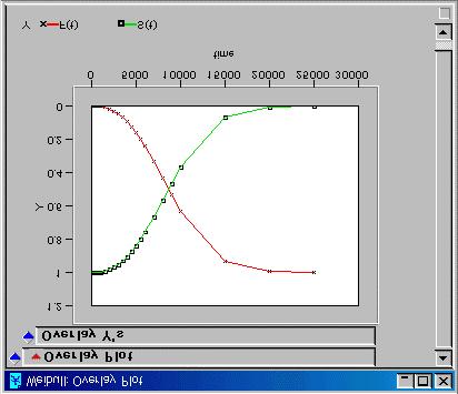
37 time Weibull time f(t),f(t),s(t) h1(t) 2.5 h2(t) 1.0 h3(t)

38 1.1 1.Overlay Plot 2.

39 1.2 3.f(t) 1.Time 4.Y 2.X 5.OK

40 1.3 1.Connect Thru Missing 2.
41
 1")
42 1 Weibull.JMP h(t) 1 1 1
43 Calculator Cols Column Info. Current Properties Formula Edit Formula, 2 Col Name
44 LnNormal.JMP,, f t ( ) 1 1 logt = exp σt 2π 2 σ µ 2
45 ( x µ ) 2 1 f( x) = exp, x 2 < <+ σ 2π 2σ ( t µ ) 2 1 x 2 σ 2π 2σ F( x) = exp dt, < x<+
46 ( ) ( ) f t = λexp λt t 0, λ> 0 ( ) ( λ ) F t f(t) = 1 exp t t 0, λ > 0 t
47 ( ln t µ ) f() t = exp t 0 2 σ 2π t > 2σ ( ) F t ( ln x µ ) 2 1 t 1 = exp dxt 0 2 > 0 σ 2π x 2σ f(t)
48
49 49
50
51 V4, weibull,3 weibull,, Weibull
52 Weibull S t t = 1 F t = exp α ( ) ( ) ( ) log S t t = α β β t α log S( t) = log{ log ( )} S t β log t = α log logs t = β logα + β logt { ( )} β
53 2 Weibull.JMP 2 Weibull Column 1 Calculator,-lnS(t) Analyze Fit Y X,X time,y -lns(t)

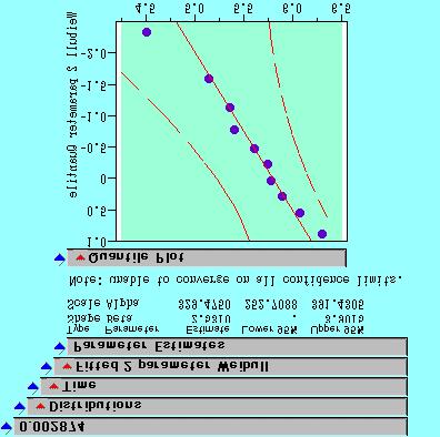
54 2 Weibull.JMP Weibull time S(time)
55 Wiring JMP Time Analyze Distribution Fit DistributionWeibull
56 Weibull Weibull
57 Part II Survival 57
58
59
60
61
62
63 Survival Survival Distribution Kaplan-Meier Parametric Regression Proportional Hazards Cox Recurrence
64 Weibull 64
65 (censor) (censor) 1. 2.
66 Censor Censor
67 3 Wiring.JMP, Survival Disuribution Survival Weibull Weibull Weibull
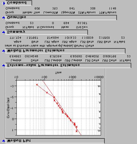
68 (Al ). Time( ) Censor( ) Distribution
69 3.1 1.Survival Distribution 2.Time 3.Y 4.OK

70 3.2 Weibull Weibull Plot Weibull Fit

71 3.3 Weibull
72 3.4 1.Survival Distribution 3.Y 2.Time 4.Censor 6.OK 5.Censor


73 3.5 1.Plot Options Show Confid Interval 2. Kaplan-Meier, 95


74 3.6 Weibull 1.Weibull Plot,Weibull Fit 2.Weibull 3.Save Estimates
75 3.7
76 3 Wiring.JMP Extreme-value Parameter Estimates Weibull Parameter Estimates Weibull 95 Delta Weibull Beta=1/Delta Lambda Weibull 63.2 Alpha=e Lambda Weibull Exponential Plot LogNormal Plot
77 Kaplan Meier n ( ) { t i} i= 1 t i d i t i n i,, ( ) ˆ d d d d S t = = 1 n n i L n1 n2 nn ti < t ni ( ) 1 2
78 Kaplan Meier ˆ d d d d S t = = 1 n n i L n1 n2 nn ti < t ni ( ) 1 2, n ˆ d i logs( t) = log 1 i= 1 n log ˆ d V S = V log 1 i= 1 n n i i i
79 Kaplan-Meier 1 V log Sˆ V Sˆ ˆ 2 S, V log Sˆ = V Sˆ = Sˆ 2 n d i di V log 1 = ni ni ni di d n i i= 1 ni ni i di n n d ( ) i= 1 i i i ( d ) ( )
80 Kaplan-Meier Sˆ = n 1 n i= 1 1 n d i ( ) 1 / 1 V Sˆ = Sˆ Sˆ n
81 t i ht ( ) i Dt = t, t ( ) i i t, n i + Dt 0 H t ( ) i i tk = k= 1 t 1 Ht ( i) = k= 1 i
82 ) Excel
83 =count( ) If F(t) A$1-C3+1 E3/D3 If
84 MON j = MON + j 1 n+ 1 MON n+ 1 ( i 1) MON(Mean Order Number) F(t) j 1
85
86
87 87
88 1 Kaplan-Meier Wilcoxon
89 Wilcoxon
90
91 j ( j 1,2,, k) = L t j t j 1 d 1 11 n11 d11 n d 11 1j n1j d1j n1j 1 d1k n1k d1k n1k L L 2 d 2 d 21 n21 d21 n 21 2 j n2 j d2 j n2 j 2 d2 k n2k d2k n2k d n d n d n d n d n d n j j j j j k k k k m = d n / n, m = d n / n 1j j 1j j 2 j j 2 j j
92 ( ) ( 1) n n n-d n n d n d v d n n n n 1j 1j j j 1j 2j j j j 1 j = j 1 = 2 j j n-1 j j j ( ) ( 1) n n n-d n n d n d v d n n n n 2 j = j 2 j 2j j j 1j 2j j j j 1 = 2 j j n-1 j j j n= d, p= n / n j 1 j j,
93 δ = d m, δ = d m 1j 1j 1j 2 j 2 j 2 j δ1j = ( d1j m1j), δ2j = ( d2j m2j)
94 n 1 n 1j n n 1j j δ1j = d1j dj = d1j = n j n j n n j n n v = 1j 2 j 1 2 n j 1 j 1 j
95 n δ1j = wj( d m 1j 1j) = wj d 1j n ( ) ( nj 1) n1jn2jd j nj dj v1 j = wj, wj = 1 n δ ( ) 1 1 j = w d m = w d 1j 1 j j j j j ( ) ( nj 1) n n d n d v w w n n 1j 2 j j j j 1 j = j, j = j j n 1 j j 1 j n j
96 δ n 1 n n = n = w d = ( nd n ) = S 1j 1 j 2 n 1 j 1j j j 1j n j ( ) ( nj 1) n n d n d 1j 2 j j j j 1j = wj = n1jn2 j n j j 1j 2j 1 j

97
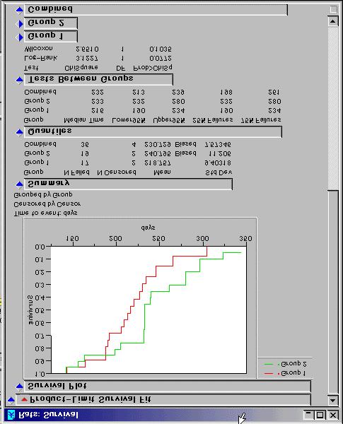
98 4 Rats.JMP, Survival Time Modeling 2 Survival
99 2 day Group ) Censor )

100 4.1 1.Survival Distribution 2.days 3.Y 4.Censor 6.Group 8.OK 5.Censor 7.Grouping
101


102 4.3 ( ) Plot Options Show Conbined
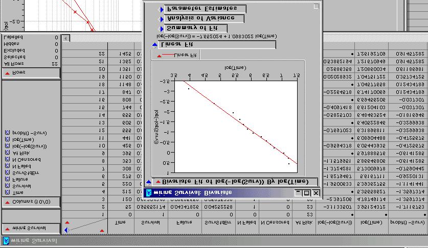
103 4 Rats.JMP
104 days. 2Survival Survival=(At Risk - N Failed)/At Risk 3Failure Survival+Failure=1 SurvStdErr(Survival Standard Error)
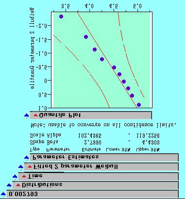
105 N Failed 1 N Censored 1 At Risk Quantiles Mean StdDev Standard Deviation
106 PWB JMP Weibull
107 PWB
108
109
110
111 111
112 (, )
113
114 1
115 ,
116 ( ),m=1( ),
117 A
118 ( ) ( ) No. time x; V d1: d i n M M M M M M M M M M
119 5 Unit.JMP Survival Time Modeling Survival Omit
120 Unit.JMP
121 2 time ) failure ) 2 Condenser Relay

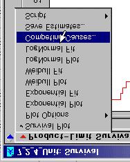

122 5.1 1.Survival Distribution 2.time 4.OK 3.Y 5.Competing Causes 6.Falure

123 5.2 Weibull Plot Weibull


124 1.Omit Causes 5.3 Weibull Weibull 2.Condenser 3.OK
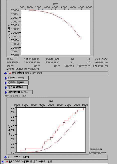
125 5.4
126 5 Unit.JMP Competing Causes condenser Omit condenser Failure Grouping
127 Part III 127
128 1
129 S ( ) a S ( t) o t = a S t = as t a ( ) ( ) o h ( ) a h ( t) o t = a S t = S t a ( ) ( ) a o
130 Weibull ( ) ( ) a Sa t = S0 t lns t = lns t lns t = ln S t a ( ) ( ) ( ) ( ) 0 a 0 { ( )} ( ) a { a } ( ) 0 0 { } ln lns t = ln lns t = ln aln S t a β t = lna+ ln = ( βlnα + lna) + β ln t α ln a,, ( ) a
131 Weibull, { S ( t) } S ( t) ln ln ln ln a { } β t t = lna+ ln ln = ln a α α Weibull Weibull 0 β
132 Ht ( ) = βt Ht ( ) = βln ( t/ α) α Ht ( ) e βt β Ht = t/ α = ( ) ( ) β
133 h ( ) ( ) ( ) x t = h0 t exp bx h 0 (t) x 0 h 0 (t) b hi( t) h0 ( t) exp( bxi) = = exp{ b( x )} i xj i j h ( t) h t exp bx j 0 ( ) ( ) j
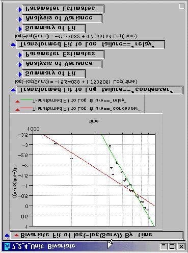
134 PWB JMP Survival Distribution Y Time1 Grouping /kt K-M Log(Time) Log(-logS(t)) Group 1/kT
 log Ht () = 12.98731+ 2.")
135 Weibull log Ht () = log( Time) log Ht () = log( Time) log Ht () = log( Time)
136 1/kT=32.** ( ) 33.** 32.** = ** 32.** = kt COX
137 COX ,COX
138 L,,,
139 , 2 2
140 Arrhenius Life= exp b + b 1/ kt Eˆ = b, k = { ( )} a 1 Life= exp { ( ) } ˆ b0 + b1 ln 2 T b1 = 1/ θ Eyring Life/ T = exp{ b + b ( 1/ kt) } Eˆ a = b (n) Life= exp{ b ( )} ˆ 0 + b1 ln T n= b
141 t Log-Normal Distribution Acceleated x
142
143 R= R0 exp B T T 0 α = 1 R log y = b + b x R dr dt T x = 1/ ( 273+ t) T = B T logyˆ = log x R 1 yˆ R = exp xt 2 T
144
145
146 PWB JMP Weibull
147 PWB
148 PWB,?
149 PWB?,
150 PWB!!!
151 PWB
152 ( ),
153 6 Creep.JMP 1 ( ), Survival Time Modeling (Weibull )
154 . temp ( ) 1/ time Censor( ) Life= exp(b 0 +b 1 /(273+temp)) exp(b 0 +b 1 /T)
155
156 T ( C + log L) = Q L = exp( Q/T - C) T L
157 Larson-Miller Larson-Miller
158

159 8.Run Mode Proportional Hazards 2.time 3.Time to Even 5.Censor 4.Censor 6.1/T 7.Add

160 Risk = h h ( t) ( t) ( ) { } = exp =

161 8.Weibull 9.Run Model 5.Censor Parametric Regression 2.time 3.Time to Event 4.Censor 6.1/T 7.Add

162 6.4 Weibull =1/ 95 1 (1 ), 1 ˆ α = exp T 1.844
163 Columns 2 2., 3.Formula, 1 αˆ = exp T ln( time) ln ( ) res = exp 4. Survival Distribution,Y,Censor Censor,Weibull Weibull

164 6.5 Weibull
165 6 Creep.JMP Parameter Estimates 1/ 95. RiskRatio (exp( )). Baseline Survival at time. weibull Parameter Estimates 1/
166 { 5 T } α ˆ = exp / ˆ exp A F 1 1 T1 T2 5 = ˆ h ( t) exp HR = = h ( ) 2 t T 1 T 2
167 167
168 Survival fit model
169 h i 1 0 exp( β1 Ti Ea 1 = h 0( ti ) exp( β1 / Ti ) = h0 ( ti ) exp( ) k T ( t) = h ( t) β + β ) = h ( t) exp( β ) exp( / T ) i E = b k a 1 i AF = 1 exp β1 Ti 1 T j = E exp k a 1 Ti 1 T j
170 ( 1/ T ) ( ) i + β2 Si β RHi zi = β 0 + β1 ln + 3 ( ) ( ) ( ) ( ) β t h t exp exp / T S ( RH ) 2 = β β β h i 0 j 0 1 i i exp 3 i AF S β 2 i = exp β S 1 exp j Ti T 3 j 1 1 { β ( S S )} i j
171 7 Reliable.JMP ( ) Survival Weibull
172 .. Glue( )---- Temp( ) 1/(k ) RH( ) Day Censor( )
173 7.1.Day 1.Parametric Regression 3.Time to Event 8.Weibull 9.Run Model 5.Censor 7.Add.Censor 6.glue,1/kT,RH

174 7.2 Weibull
175 7 Reliable.JMP 1/ = exp( )= exp( /kt rh) (eV) (eV)
176 LnReg.JMP,,,,,, / T,, 3., 4.
177 1 1 L exp β 0 exp β 1 exp 2 log10 T β T σ = ln L = C + 1 log T + 1 β β σ T ε N(0, 2 ) σ T T ˆ 4 = exp exp log10 L
178
179
180
181 L T E a n = expa exp T I kt B ( ) ( ) E a n L= expa exp T I kt B ( ) ( ) temp 1/ k T, T ln T I ln I B k k
182 1/(k B T) ln( ) ln( T) m ηˆ = exp T kt B I ( ) ( )
183 1/(k B T) ln( ) ln( T) m ηˆ = T exp T I kt B ( ) ( )
184 184
185 ( ) Prentice1974.JMP
186 VA Lung Cancer.JMP. COX,
2 H23 BioS (i) data d1; input group patno t sex censor; cards;
 data d1; input group patno t sex censor; cards;") H BioS (i) data d1; input group patno t sex censor; cards; 0 1 0 0 0 0 1 0 1 1 0 4 4 0 1 0 5 5 1 1 0 6 5 1 1 0 7 10 1 0 0 8 15 0 1 0 9 15 0 1 0 10 4 1 0 0 11 4 1 0 1 1 5 1 0 1 1 7 0 1 1 14 8 1 0 1 15 8
H BioS (i) data d1; input group patno t sex censor; cards; 0 1 0 0 0 0 1 0 1 1 0 4 4 0 1 0 5 5 1 1 0 6 5 1 1 0 7 10 1 0 0 8 15 0 1 0 9 15 0 1 0 10 4 1 0 0 11 4 1 0 1 1 5 1 0 1 1 7 0 1 1 14 8 1 0 1 15 8
201711grade1ouyou.pdf
 2017 11 26 1 2 52 3 12 13 22 23 32 33 42 3 5 3 4 90 5 6 A 1 2 Web Web 3 4 1 2... 5 6 7 7 44 8 9 1 2 3 1 p p >2 2 A 1 2 0.6 0.4 0.52... (a) 0.6 0.4...... B 1 2 0.8-0.2 0.52..... (b) 0.6 0.52.... 1 A B 2
untitled
 18 1 2,000,000 2,000,000 2007 2 2 2008 3 31 (1) 6 JCOSSAR 2007pp.57-642007.6. LCC (1) (2) 2 10mm 1020 14 12 10 8 6 4 40,50,60 2 0 1998 27.5 1995 1960 40 1) 2) 3) LCC LCC LCC 1 1) Vol.42No.5pp.29-322004.5.
総合薬学講座 生物統計の基礎
 2013 10 22 ( ) 2013 10 22 1 / 40 p.682 1. 2. 3 2 t Mann Whitney U ). 4 χ 2. 5. 6 Dunnett Tukey. 7. 8 Kaplan Meier.. U. ( ) 2013 10 22 2 / 40 1 93 ( 20 ) 230. a t b c χ 2 d 1.0 +1.0 e, b ( ) e ( ) ( ) 2013
) ] [ h m x + y + + V x) φ = Eφ 1) z E = i h t 13) x << 1) N n n= = N N + 1) 14) N n n= = N N + 1)N + 1) 6 15) N n 3 n= = 1 4 N N + 1) 16) N n 4
![) ] [ h m x + y + + V x) φ = Eφ 1) z E = i h t 13) x << 1) N n n= = N N + 1) 14) N n n= = N N + 1)N + 1) 6 15) N n 3 n= = 1 4 N N + 1) 16) N n 4](/thumbs/92/107866707.jpg ") ] [ h m x + y + + V x) φ = Eφ 1) z E = i h t 13) x << 1) N n n= = N N + 1) 14) N n n= = N N + 1)N + 1) 6 15) N n 3 n= = 1 4 N N + 1) 16) N n 4") 1. k λ ν ω T v p v g k = π λ ω = πν = π T v p = λν = ω k v g = dω dk 1) ) 3) 4). p = hk = h λ 5) E = hν = hω 6) h = h π 7) h =6.6618 1 34 J sec) hc=197.3 MeV fm = 197.3 kev pm= 197.3 ev nm = 1.97 1 3 ev
1. k λ ν ω T v p v g k = π λ ω = πν = π T v p = λν = ω k v g = dω dk 1) ) 3) 4). p = hk = h λ 5) E = hν = hω 6) h = h π 7) h =6.6618 1 34 J sec) hc=197.3 MeV fm = 197.3 kev pm= 197.3 ev nm = 1.97 1 3 ev
Part () () Γ Part ,
 () Γ Part ,") Contents a 6 6 6 6 6 6 6 7 7. 8.. 8.. 8.3. 8 Part. 9. 9.. 9.. 3. 3.. 3.. 3 4. 5 4.. 5 4.. 9 4.3. 3 Part. 6 5. () 6 5.. () 7 5.. 9 5.3. Γ 3 6. 3 6.. 3 6.. 3 6.3. 33 Part 3. 34 7. 34 7.. 34 7.. 34 8. 35
Contents a 6 6 6 6 6 6 6 7 7. 8.. 8.. 8.3. 8 Part. 9. 9.. 9.. 3. 3.. 3.. 3 4. 5 4.. 5 4.. 9 4.3. 3 Part. 6 5. () 6 5.. () 7 5.. 9 5.3. Γ 3 6. 3 6.. 3 6.. 3 6.3. 33 Part 3. 34 7. 34 7.. 34 7.. 34 8. 35
S I. dy fx x fx y fx + C 3 C dy fx 4 x, y dy v C xt y C v e kt k > xt yt gt [ v dt dt v e kt xt v e kt + C k x v + C C k xt v k 3 r r + dr e kt S dt d
 S I.. http://ayapin.film.s.dendai.ac.jp/~matuda /TeX/lecture.html PDF PS.................................... 3.3.................... 9.4................5.............. 3 5. Laplace................. 5....
S I. dy fx x fx y fx + C 3 C vt dy fx 4 x, y dy yt gt + Ct + C dt v e kt xt v e kt + C k x v k + C C xt v k 3 r r + dr e kt S Sr πr dt d v } dt k e kt
 S I. x yx y y, y,. F x, y, y, y,, y n http://ayapin.film.s.dendai.ac.jp/~matuda n /TeX/lecture.html PDF PS yx.................................... 3.3.................... 9.4................5..............
こんにちは由美子です
 Sample size power calculation Sample Size Estimation AZTPIAIDS AIDSAZT AIDSPI AIDSRNA AZTPr (S A ) = π A, PIPr (S B ) = π B AIDS (sampling)(inference) π A, π B π A - π B = 0.20 PI 20 20AZT, PI 10 6 8 HIV-RNA
5 5.1 E 1, E 2 N 1, N 2 E tot N tot E tot = E 1 + E 2, N tot = N 1 + N 2 S 1 (E 1, N 1 ), S 2 (E 2, N 2 ) E 1, E 2 S tot = S 1 + S 2 2 S 1 E 1 = S 2 E
, S 2 (E 2, N 2 ) E 1, E 2 S tot = S 1 + S 2 2 S 1 E 1 = S 2 E") 5 5.1 E 1, E 2 N 1, N 2 E tot N tot E tot = E 1 + E 2, N tot = N 1 + N 2 S 1 (E 1, N 1 ), S 2 (E 2, N 2 ) E 1, E 2 S tot = S 1 + S 2 2 S 1 E 1 = S 2 E 2, S 1 N 1 = S 2 N 2 2 (chemical potential) µ S N
5 5.1 E 1, E 2 N 1, N 2 E tot N tot E tot = E 1 + E 2, N tot = N 1 + N 2 S 1 (E 1, N 1 ), S 2 (E 2, N 2 ) E 1, E 2 S tot = S 1 + S 2 2 S 1 E 1 = S 2 E 2, S 1 N 1 = S 2 N 2 2 (chemical potential) µ S N
( ) 2.1. C. (1) x 4 dx = 1 5 x5 + C 1 (2) x dx = x 2 dx = x 1 + C = 1 2 x + C xdx (3) = x dx = 3 x C (4) (x + 1) 3 dx = (x 3 + 3x 2 + 3x +
 2.1. C. (1) x 4 dx = 1 5 x5 + C 1 (2) x dx = x 2 dx = x 1 + C = 1 2 x + C xdx (3) = x dx = 3 x C (4) (x + 1) 3 dx = (x 3 + 3x 2 + 3x +") (.. C. ( d 5 5 + C ( d d + C + C d ( d + C ( ( + d ( + + + d + + + + C (5 9 + d + d tan + C cos (sin (6 sin d d log sin + C sin + (7 + + d ( + + + + d log( + + + C ( (8 d 7 6 d + 6 + C ( (9 ( d 6 + 8 d
(.. C. ( d 5 5 + C ( d d + C + C d ( d + C ( ( + d ( + + + d + + + + C (5 9 + d + d tan + C cos (sin (6 sin d d log sin + C sin + (7 + + d ( + + + + d log( + + + C ( (8 d 7 6 d + 6 + C ( (9 ( d 6 + 8 d
meiji_resume_1.PDF
 β β β (q 1,q,..., q n ; p 1, p,..., p n ) H(q 1,q,..., q n ; p 1, p,..., p n ) Hψ = εψ ε k = k +1/ ε k = k(k 1) (x, y, z; p x, p y, p z ) (r; p r ), (θ; p θ ), (ϕ; p ϕ ) ε k = 1/ k p i dq i E total = E
1 (Berry,1975) 2-6 p (S πr 2 )p πr 2 p 2πRγ p p = 2γ R (2.5).1-1 : : : : ( ).2 α, β α, β () X S = X X α X β (.1) 1 2
 2-6 p (S πr 2 )p πr 2 p 2πRγ p p = 2γ R (2.5).1-1 : : : : ( ).2 α, β α, β () X S = X X α X β (.1) 1 2") 2005 9/8-11 2 2.2 ( 2-5) γ ( ) γ cos θ 2πr πρhr 2 g h = 2γ cos θ ρgr (2.1) γ = ρgrh (2.2) 2 cos θ θ cos θ = 1 (2.2) γ = 1 ρgrh (2.) 2 2. p p ρgh p ( ) p p = p ρgh (2.) h p p = 2γ r 1 1 (Berry,1975) 2-6
2005 9/8-11 2 2.2 ( 2-5) γ ( ) γ cos θ 2πr πρhr 2 g h = 2γ cos θ ρgr (2.1) γ = ρgrh (2.2) 2 cos θ θ cos θ = 1 (2.2) γ = 1 ρgrh (2.) 2 2. p p ρgh p ( ) p p = p ρgh (2.) h p p = 2γ r 1 1 (Berry,1975) 2-6
5 Armitage x 1,, x n y i = 10x i + 3 y i = log x i {x i } {y i } 1.2 n i i x ij i j y ij, z ij i j 2 1 y = a x + b ( cm) x ij (i j )
 x ij (i j )") 5 Armitage. x,, x n y i = 0x i + 3 y i = log x i x i y i.2 n i i x ij i j y ij, z ij i j 2 y = a x + b 2 2. ( cm) x ij (i j ) (i) x, x 2 σ 2 x,, σ 2 x,2 σ x,, σ x,2 t t x * (ii) (i) m y ij = x ij /00 y
5 Armitage. x,, x n y i = 0x i + 3 y i = log x i x i y i.2 n i i x ij i j y ij, z ij i j 2 y = a x + b 2 2. ( cm) x ij (i j ) (i) x, x 2 σ 2 x,, σ 2 x,2 σ x,, σ x,2 t t x * (ii) (i) m y ij = x ij /00 y
.. ( )T p T = p p = T () T x T N P (X < x T ) N = ( T ) N (2) ) N ( P (X x T ) N = T (3) T N P T N P 0
T p T = p p = T () T x T N P (X < x T ) N = ( T ) N (2) ) N ( P (X x T ) N = T (3) T N P T N P 0") 20 5 8..................................................2.....................................3 L.....................................4................................. 2 2. 3 2. (N ).........................................
20 5 8..................................................2.....................................3 L.....................................4................................. 2 2. 3 2. (N ).........................................
k2 ( :35 ) ( k2) (GLM) web web 1 :
 ( k2) (GLM) web web 1 :") 2012 11 01 k2 (2012-10-26 16:35 ) 1 6 2 (2012 11 01 k2) (GLM) kubo@ees.hokudai.ac.jp web http://goo.gl/wijx2 web http://goo.gl/ufq2 1 : 2 2 4 3 7 4 9 5 : 11 5.1................... 13 6 14 6.1......................
2012 11 01 k2 (2012-10-26 16:35 ) 1 6 2 (2012 11 01 k2) (GLM) kubo@ees.hokudai.ac.jp web http://goo.gl/wijx2 web http://goo.gl/ufq2 1 : 2 2 4 3 7 4 9 5 : 11 5.1................... 13 6 14 6.1......................
 http://www.ike-dyn.ritsumei.ac.jp/ hyoo/wave.html 1 1, 5 3 1.1 1..................................... 3 1.2 5.1................................... 4 1.3.......................... 5 1.4 5.2, 5.3....................
II III II 1 III ( ) [2] [3] [1] 1 1:
![II III II 1 III ( ) [2] [3] [1] 1 1:](/thumbs/103/160503680.jpg "II III II 1 III ( ) [2] [3] [1] 1 1:") 2015 4 16 1. II III II 1 III () [2] [3] 2013 11 18 [1] 1 1: [5] [6] () [7] [1] [1] 1998 4 2008 8 2014 8 6 [1] [1] 2 3 4 5 2. 2.1. t Dt L DF t A t (2.1) A t = Dt L + Dt F (2.1) 3 2 1 2008 9 2008 8 2008
2015 4 16 1. II III II 1 III () [2] [3] 2013 11 18 [1] 1 1: [5] [6] () [7] [1] [1] 1998 4 2008 8 2014 8 6 [1] [1] 2 3 4 5 2. 2.1. t Dt L DF t A t (2.1) A t = Dt L + Dt F (2.1) 3 2 1 2008 9 2008 8 2008
1 Tokyo Daily Rainfall (mm) Days (mm)
 Days (mm)") ( ) r-taka@maritime.kobe-u.ac.jp 1 Tokyo Daily Rainfall (mm) 0 100 200 300 0 10000 20000 30000 40000 50000 Days (mm) 1876 1 1 2013 12 31 Tokyo, 1876 Daily Rainfall (mm) 0 50 100 150 0 100 200 300 Tokyo,
( ) r-taka@maritime.kobe-u.ac.jp 1 Tokyo Daily Rainfall (mm) 0 100 200 300 0 10000 20000 30000 40000 50000 Days (mm) 1876 1 1 2013 12 31 Tokyo, 1876 Daily Rainfall (mm) 0 50 100 150 0 100 200 300 Tokyo,
*1 * Wilcoxon 2 2 t t t t d t M t N t M t n t N t n t N t d t N t t at ri
 Wilcoxon H23 BioS 1 Wilcoxon 2 2.1 1 2 1 0 1 1 5 0 1 2 7 0 1 3 8 1 1 4 12 0 2 5 2 0 2 6 3 1 2 7 4 1 2 8 10 0 Wilcoxon 2.2 S 1 t S 2 t Wilcoxon H 0 H 1 H 0 : S 1 t S 2 t H 1 : S 1 t S 2 t 1 *1 *2 2.3 2.3.1
³ÎΨÏÀ
 2017 12 12 Makoto Nakashima 2017 12 12 1 / 22 2.1. C, D π- C, D. A 1, A 2 C A 1 A 2 C A 3, A 4 D A 1 A 2 D Makoto Nakashima 2017 12 12 2 / 22 . (,, L p - ). Makoto Nakashima 2017 12 12 3 / 22 . (,, L p
,,,17,,, ( ),, E Q [S T F t ] < S t, t [, T ],,,,,,,,
![,,,17,,, ( ),, E Q [S T F t ] < S t, t [, T ],,,,,,,,](/thumbs/91/105754403.jpg ",,,17,,, ( ),, E Q [S T F t ] < S t, t [, T ],,,,,,,,") 14 5 1 ,,,17,,,194 1 4 ( ),, E Q [S T F t ] < S t, t [, T ],,,,,,,, 1 4 1.1........................................ 4 5.1........................................ 5.........................................
14 5 1 ,,,17,,,194 1 4 ( ),, E Q [S T F t ] < S t, t [, T ],,,,,,,, 1 4 1.1........................................ 4 5.1........................................ 5.........................................
9 5 ( α+ ) = (α + ) α (log ) = α d = α C d = log + C C 5. () d = 4 d = C = C = 3 + C 3 () d = d = C = C = 3 + C 3 =
 = (α + ) α (log ) = α d = α C d = log + C C 5. () d = 4 d = C = C = 3 + C 3 () d = d = C = C = 3 + C 3 =") 5 5. 5.. A II f() f() F () f() F () = f() C (F () + C) = F () = f() F () + C f() F () G() f() G () = F () 39 G() = F () + C C f() F () f() F () + C C f() f() d f() f() C f() f() F () = f() f() f() d =
5 5. 5.. A II f() f() F () f() F () = f() C (F () + C) = F () = f() F () + C f() F () G() f() G () = F () 39 G() = F () + C C f() F () f() F () + C C f() f() d f() f() C f() f() F () = f() f() f() d =
gr09.dvi
 .1, θ, ϕ d = A, t dt + B, t dtd + C, t d + D, t dθ +in θdϕ.1.1 t { = f1,t t = f,t { D, t = B, t =.1. t A, tdt e φ,t dt, C, td e λ,t d.1.3,t, t d = e φ,t dt + e λ,t d + dθ +in θdϕ.1.4 { = f1,t t = f,t {
positron 1930 Dirac 1933 Anderson m 22Na(hl=2.6years), 58Co(hl=71days), 64Cu(hl=12hour) 68Ge(hl=288days) MeV : thermalization m psec 100
, 58Co(hl=71days), 64Cu(hl=12hour) 68Ge(hl=288days) MeV : thermalization m psec 100") positron 1930 Dirac 1933 Anderson m 22Na(hl=2.6years), 58Co(hl=71days), 64Cu(hl=12hour) 68Ge(hl=288days) 0.5 1.5MeV : thermalization 10 100 m psec 100psec nsec E total = 2mc 2 + E e + + E e Ee+ Ee-c mc
positron 1930 Dirac 1933 Anderson m 22Na(hl=2.6years), 58Co(hl=71days), 64Cu(hl=12hour) 68Ge(hl=288days) 0.5 1.5MeV : thermalization 10 100 m psec 100psec nsec E total = 2mc 2 + E e + + E e Ee+ Ee-c mc
²¾ÁÛ¾õ¶·É¾²ÁË¡¤Î¤¿¤á¤Î¥Ñ¥Ã¥±¡¼¥¸DCchoice ¡Ê»ÃÄêÈÇ¡Ë
 DCchoice ( ) R 2013 2013 11 30 DCchoice package R 2013/11/30 1 / 19 1 (CV) CV 2 DCchoice WTP 3 DCchoice package R 2013/11/30 2 / 19 (Contingent Valuation; CV) WTP CV WTP WTP 1 1989 2 DCchoice package R
10:30 12:00 P.G. vs vs vs 2
 1 10:30 12:00 P.G. vs vs vs 2 LOGIT PROBIT TOBIT mean median mode CV 3 4 5 0.5 1000 6 45 7 P(A B) = P(A) + P(B) - P(A B) P(B A)=P(A B)/P(A) P(A B)=P(B A) P(A) P(A B) P(A) P(B A) P(B) P(A B) P(A) P(B) P(B
数学概論I
 {a n } M >0 s.t. a n 5 M for n =1, 2,... lim n a n = α ε =1 N s.t. a n α < 1 for n > N. n > N a n 5 a n α + α < 1+ α. M := max{ a 1,..., a N, 1+ α } a n 5 M ( n) 1 α α 1+ α t a 1 a N+1 a N+2 a 2 1 a n
chap9.dvi
 9 AR (i) (ii) MA (iii) (iv) (v) 9.1 2 1 AR 1 9.1.1 S S y j = (α i + β i j) D ij + η j, η j = ρ S η j S + ε j (j =1,,T) (1) i=1 {ε j } i.i.d(,σ 2 ) η j (j ) D ij j i S 1 S =1 D ij =1 S>1 S =4 (1) y j =
2 1,2, , 2 ( ) (1) (2) (3) (4) Cameron and Trivedi(1998) , (1987) (1982) Agresti(2003)
 (1) (2) (3) (4) Cameron and Trivedi(1998) , (1987) (1982) Agresti(2003)") 3 1 1 1 2 1 2 1,2,3 1 0 50 3000, 2 ( ) 1 3 1 0 4 3 (1) (2) (3) (4) 1 1 1 2 3 Cameron and Trivedi(1998) 4 1974, (1987) (1982) Agresti(2003) 3 (1)-(4) AAA, AA+,A (1) (2) (3) (4) (5) (1)-(5) 1 2 5 3 5 (DI)
3 1 1 1 2 1 2 1,2,3 1 0 50 3000, 2 ( ) 1 3 1 0 4 3 (1) (2) (3) (4) 1 1 1 2 3 Cameron and Trivedi(1998) 4 1974, (1987) (1982) Agresti(2003) 3 (1)-(4) AAA, AA+,A (1) (2) (3) (4) (5) (1)-(5) 1 2 5 3 5 (DI)
untitled
 3 3. (stochastic differential equations) { dx(t) =f(t, X)dt + G(t, X)dW (t), t [,T], (3.) X( )=X X(t) : [,T] R d (d ) f(t, X) : [,T] R d R d (drift term) G(t, X) : [,T] R d R d m (diffusion term) W (t)
1 No.1 5 C 1 I III F 1 F 2 F 1 F 2 2 Φ 2 (t) = Φ 1 (t) Φ 1 (t t). = Φ 1(t) t = ( 1.5e 0.5t 2.4e 4t 2e 10t ) τ < 0 t > τ Φ 2 (t) < 0 lim t Φ 2 (t) = 0
 = Φ 1 (t) Φ 1 (t t). = Φ 1(t) t = ( 1.5e 0.5t 2.4e 4t 2e 10t ) τ < 0 t > τ Φ 2 (t) < 0 lim t Φ 2 (t) = 0") 1 No.1 5 C 1 I III F 1 F 2 F 1 F 2 2 Φ 2 (t) = Φ 1 (t) Φ 1 (t t). = Φ 1(t) t = ( 1.5e 0.5t 2.4e 4t 2e 10t ) τ < 0 t > τ Φ 2 (t) < 0 lim t Φ 2 (t) = 0 0 < t < τ I II 0 No.2 2 C x y x y > 0 x 0 x > b a dx
1 No.1 5 C 1 I III F 1 F 2 F 1 F 2 2 Φ 2 (t) = Φ 1 (t) Φ 1 (t t). = Φ 1(t) t = ( 1.5e 0.5t 2.4e 4t 2e 10t ) τ < 0 t > τ Φ 2 (t) < 0 lim t Φ 2 (t) = 0 0 < t < τ I II 0 No.2 2 C x y x y > 0 x 0 x > b a dx
1 1.1 ( ). z = a + bi, a, b R 0 a, b 0 a 2 + b 2 0 z = a + bi = ( ) a 2 + b 2 a a 2 + b + b 2 a 2 + b i 2 r = a 2 + b 2 θ cos θ = a a 2 + b 2, sin θ =
. z = a + bi, a, b R 0 a, b 0 a 2 + b 2 0 z = a + bi = ( ) a 2 + b 2 a a 2 + b + b 2 a 2 + b i 2 r = a 2 + b 2 θ cos θ = a a 2 + b 2, sin θ =") 1 1.1 ( ). z = + bi,, b R 0, b 0 2 + b 2 0 z = + bi = ( ) 2 + b 2 2 + b + b 2 2 + b i 2 r = 2 + b 2 θ cos θ = 2 + b 2, sin θ = b 2 + b 2 2π z = r(cos θ + i sin θ) 1.2 (, ). 1. < 2. > 3. ±,, 1.3 ( ). A
1 1.1 ( ). z = + bi,, b R 0, b 0 2 + b 2 0 z = + bi = ( ) 2 + b 2 2 + b + b 2 2 + b i 2 r = 2 + b 2 θ cos θ = 2 + b 2, sin θ = b 2 + b 2 2π z = r(cos θ + i sin θ) 1.2 (, ). 1. < 2. > 3. ±,, 1.3 ( ). A
.. F x) = x ft)dt ), fx) : PDF : probbility density function) F x) : CDF : cumultive distribution function F x) x.2 ) T = µ p), T : ) p : x p p = F x
 = x ft)dt ), fx) : PDF : probbility density function) F x) : CDF : cumultive distribution function F x) x.2 ) T = µ p), T : ) p : x p p = F x") 203 7......................................2................................................3.....................................4 L.................................... 2.5.................................
203 7......................................2................................................3.....................................4 L.................................... 2.5.................................
構造と連続体の力学基礎
 II 37 Wabash Avenue Bridge, Illinois 州 Winnipeg にある歩道橋 Esplanade Riel 橋6 6 斜張橋である必要は多分無いと思われる すぐ横に道路用桁橋有り しかも塔基部のレストランは 8 年には営業していなかった 9 9. 9.. () 97 [3] [5] k 9. m w(t) f (t) = f (t) + mg k w(t) Newton
[ ] (Ising model) 2 i S i S i = 1 (up spin : ) = 1 (down spin : ) (4.38) s z = ±1 4 H 0 = J zn/2 i,j S i S j (4.39) i, j z 5 2 z = 4 z = 6 3
![[ ] (Ising model) 2 i S i S i = 1 (up spin : ) = 1 (down spin : ) (4.38) s z = ±1 4 H 0 = J zn/2 i,j S i S j (4.39) i, j z 5 2 z = 4 z = 6 3](/thumbs/103/161261933.jpg "[ ] (Ising model) 2 i S i S i = 1 (up spin : ) = 1 (down spin : ) (4.38) s z = ±1 4 H 0 = J zn/2 i,j S i S j (4.39) i, j z 5 2 z = 4 z = 6 3") 4.2 4.2.1 [ ] (Ising model) 2 i S i S i = 1 (up spin : ) = 1 (down spin : ) (4.38) s z = ±1 4 H 0 = J zn/2 S i S j (4.39) i, j z 5 2 z = 4 z = 6 3 z = 6 z = 8 zn/2 1 2 N i z nearest neighbors of i j=1
4.2 4.2.1 [ ] (Ising model) 2 i S i S i = 1 (up spin : ) = 1 (down spin : ) (4.38) s z = ±1 4 H 0 = J zn/2 S i S j (4.39) i, j z 5 2 z = 4 z = 6 3 z = 6 z = 8 zn/2 1 2 N i z nearest neighbors of i j=1
lecture
 5 3 3. 9. 4. x, x. 4, f(x, ) :=x x + =4,x,.. 4 (, 3) (, 5) (3, 5), (4, 9) 95 9 (g) 4 6 8 (cm).9 3.8 6. 8. 9.9 Phsics 85 8 75 7 65 7 75 8 85 9 95 Mathematics = ax + b 6 3 (, 3) 3 ( a + b). f(a, b) ={3 (a
x (x, ) x y (, y) iy x y z = x + iy (x, y) (r, θ) r = x + y, θ = tan ( y ), π < θ π x r = z, θ = arg z z = x + iy = r cos θ + ir sin θ = r(cos θ + i s
 x y (, y) iy x y z = x + iy (x, y) (r, θ) r = x + y, θ = tan ( y ), π < θ π x r = z, θ = arg z z = x + iy = r cos θ + ir sin θ = r(cos θ + i s") ... x, y z = x + iy x z y z x = Rez, y = Imz z = x + iy x iy z z () z + z = (z + z )() z z = (z z )(3) z z = ( z z )(4)z z = z z = x + y z = x + iy ()Rez = (z + z), Imz = (z z) i () z z z + z z + z.. z
... x, y z = x + iy x z y z x = Rez, y = Imz z = x + iy x iy z z () z + z = (z + z )() z z = (z z )(3) z z = ( z z )(4)z z = z z = x + y z = x + iy ()Rez = (z + z), Imz = (z z) i () z z z + z z + z.. z
chap10.dvi
 . q {y j } I( ( L y j =Δy j = u j = C l ε j l = C(L ε j, {ε j } i.i.d.(,i q ( l= y O p ( {u j } q {C l } A l C l
I A A441 : April 15, 2013 Version : 1.1 I Kawahira, Tomoki TA (Shigehiro, Yoshida )
") I013 00-1 : April 15, 013 Version : 1.1 I Kawahira, Tomoki TA (Shigehiro, Yoshida) http://www.math.nagoya-u.ac.jp/~kawahira/courses/13s-tenbou.html pdf * 4 15 4 5 13 e πi = 1 5 0 5 7 3 4 6 3 6 10 6 17
I013 00-1 : April 15, 013 Version : 1.1 I Kawahira, Tomoki TA (Shigehiro, Yoshida) http://www.math.nagoya-u.ac.jp/~kawahira/courses/13s-tenbou.html pdf * 4 15 4 5 13 e πi = 1 5 0 5 7 3 4 6 3 6 10 6 17
) a + b = i + 6 b c = 6i j ) a = 0 b = c = 0 ) â = i + j 0 ˆb = 4) a b = b c = j + ) cos α = cos β = 6) a ˆb = b ĉ = 0 7) a b = 6i j b c = i + 6j + 8)
 a + b = i + 6 b c = 6i j ) a = 0 b = c = 0 ) â = i + j 0 ˆb = 4) a b = b c = j + ) cos α = cos β = 6) a ˆb = b ĉ = 0 7) a b = 6i j b c = i + 6j + 8)") 4 4 ) a + b = i + 6 b c = 6i j ) a = 0 b = c = 0 ) â = i + j 0 ˆb = 4) a b = b c = j + ) cos α = cos β = 6) a ˆb = b ĉ = 0 7) a b = 6i j b c = i + 6j + 8) a b a b = 6i j 4 b c b c 9) a b = 4 a b) c = 7
4 4 ) a + b = i + 6 b c = 6i j ) a = 0 b = c = 0 ) â = i + j 0 ˆb = 4) a b = b c = j + ) cos α = cos β = 6) a ˆb = b ĉ = 0 7) a b = 6i j b c = i + 6j + 8) a b a b = 6i j 4 b c b c 9) a b = 4 a b) c = 7
24 I ( ) 1. R 3 (i) C : x 2 + y 2 1 = 0 (ii) C : y = ± 1 x 2 ( 1 x 1) (iii) C : x = cos t, y = sin t (0 t 2π) 1.1. γ : [a, b] R n ; t γ(t) = (x
![24 I ( ) 1. R 3 (i) C : x 2 + y 2 1 = 0 (ii) C : y = ± 1 x 2 ( 1 x 1) (iii) C : x = cos t, y = sin t (0 t 2π) 1.1. γ : [a, b] R n ; t γ(t) = (x](/thumbs/94/118744578.jpg "24 I ( ) 1. R 3 (i) C : x 2 + y 2 1 = 0 (ii) C : y = ± 1 x 2 ( 1 x 1) (iii) C : x = cos t, y = sin t (0 t 2π) 1.1. γ : [a, b] R n ; t γ(t) = (x") 24 I 1.1.. ( ) 1. R 3 (i) C : x 2 + y 2 1 = 0 (ii) C : y = ± 1 x 2 ( 1 x 1) (iii) C : x = cos t, y = sin t (0 t 2π) 1.1. γ : [a, b] R n ; t γ(t) = (x 1 (t), x 2 (t),, x n (t)) ( ) ( ), γ : (i) x 1 (t),
24 I 1.1.. ( ) 1. R 3 (i) C : x 2 + y 2 1 = 0 (ii) C : y = ± 1 x 2 ( 1 x 1) (iii) C : x = cos t, y = sin t (0 t 2π) 1.1. γ : [a, b] R n ; t γ(t) = (x 1 (t), x 2 (t),, x n (t)) ( ) ( ), γ : (i) x 1 (t),
(1.2) T D = 0 T = D = 30 kn 1.2 (1.4) 2F W = 0 F = W/2 = 300 kn/2 = 150 kn 1.3 (1.9) R = W 1 + W 2 = = 1100 N. (1.9) W 2 b W 1 a = 0
 T D = 0 T = D = 30 kn 1.2 (1.4) 2F W = 0 F = W/2 = 300 kn/2 = 150 kn 1.3 (1.9) R = W 1 + W 2 = = 1100 N. (1.9) W 2 b W 1 a = 0") 1 1 1.1 1.) T D = T = D = kn 1. 1.4) F W = F = W/ = kn/ = 15 kn 1. 1.9) R = W 1 + W = 6 + 5 = 11 N. 1.9) W b W 1 a = a = W /W 1 )b = 5/6) = 5 cm 1.4 AB AC P 1, P x, y x, y y x 1.4.) P sin 6 + P 1 sin 45
1 1 1.1 1.) T D = T = D = kn 1. 1.4) F W = F = W/ = kn/ = 15 kn 1. 1.9) R = W 1 + W = 6 + 5 = 11 N. 1.9) W b W 1 a = a = W /W 1 )b = 5/6) = 5 cm 1.4 AB AC P 1, P x, y x, y y x 1.4.) P sin 6 + P 1 sin 45
Microsoft Word - 章末問題
 1906 R n m 1 = =1 1 R R= 8h ICP s p s HeNeArXe 1 ns 1 1 1 1 1 17 NaCl 1.3 nm 10nm 3s CuAuAg NaCl CaF - - HeNeAr 1.7(b) 2 2 2d = a + a = 2a d = 2a 2 1 1 N = 8 + 6 = 4 8 2 4 4 2a 3 4 π N πr 3 3 4 ρ = = =
TOP URL 1
 TOP URL http://amonphys.web.fc.com/ 3.............................. 3.............................. 4.3 4................... 5.4........................ 6.5........................ 8.6...........................7
untitled
 Data cleaning Original datan=8479 NCC/ptkgN=7958 NCC10x10E628 8139 NCC/kgPage 1-2) Covariate cleaningcovariate Page Page5-8 Kaplan-Meier method, Log-rank, Cox hazard model Overall survival Cumulative incidence
数学の基礎訓練I
 I 9 6 13 1 1 1.1............... 1 1................ 1 1.3.................... 1.4............... 1.4.1.............. 1.4................. 3 1.4.3........... 3 1.4.4.. 3 1.5.......... 3 1.5.1..............
医系の統計入門第 2 版 サンプルページ この本の定価 判型などは, 以下の URL からご覧いただけます. このサンプルページの内容は, 第 2 版 1 刷発行時のものです.
 医系の統計入門第 2 版 サンプルページ この本の定価 判型などは, 以下の URL からご覧いただけます. http://www.morikita.co.jp/books/mid/009192 このサンプルページの内容は, 第 2 版 1 刷発行時のものです. i 2 t 1. 2. 3 2 3. 6 4. 7 5. n 2 ν 6. 2 7. 2003 ii 2 2013 10 iii 1987
NLMIXED プロシジャを用いた生存時間解析 伊藤要二アストラゼネカ株式会社臨床統計 プログラミング グループグルプ Survival analysis using PROC NLMIXED Yohji Itoh Clinical Statistics & Programming Group, A
 NLMIXED プロシジャを用いた生存時間解析 伊藤要二アストラゼネカ株式会社臨床統計 プログラミング グループグルプ Survival analysis using PROC NLMIXED Yohji Itoh Clinical Statistics & Programming Group, AstraZeneca KK 要旨 : NLMIXEDプロシジャの最尤推定の機能を用いて 指数分布 Weibull
V(x) m e V 0 cos x π x π V(x) = x < π, x > π V 0 (i) x = 0 (V(x) V 0 (1 x 2 /2)) n n d 2 f dξ 2ξ d f 2 dξ + 2n f = 0 H n (ξ) (ii) H
 m e V 0 cos x π x π V(x) = x < π, x > π V 0 (i) x = 0 (V(x) V 0 (1 x 2 /2)) n n d 2 f dξ 2ξ d f 2 dξ + 2n f = 0 H n (ξ) (ii) H") 199 1 1 199 1 1. Vx) m e V cos x π x π Vx) = x < π, x > π V i) x = Vx) V 1 x /)) n n d f dξ ξ d f dξ + n f = H n ξ) ii) H n ξ) = 1) n expξ ) dn dξ n exp ξ )) H n ξ)h m ξ) exp ξ )dξ = π n n!δ n,m x = Vx)
199 1 1 199 1 1. Vx) m e V cos x π x π Vx) = x < π, x > π V i) x = Vx) V 1 x /)) n n d f dξ ξ d f dξ + n f = H n ξ) ii) H n ξ) = 1) n expξ ) dn dξ n exp ξ )) H n ξ)h m ξ) exp ξ )dξ = π n n!δ n,m x = Vx)
OHP.dvi
 t 0, X X t x t 0 t u u = x X (1) t t 0 u X x O 1 1 t 0 =0 X X +dx t x(x,t) x(x +dx,t). dx dx = x(x +dx,t) x(x,t) (2) dx, dx = F dx (3). F (deformation gradient tensor) t F t 0 dx dx X x O 2 2 F. (det F
i 18 2H 2 + O 2 2H 2 + ( ) 3K
 3K") i 18 2H 2 + O 2 2H 2 + ( ) 3K ii 1 1 1.1.................................. 1 1.2........................................ 3 1.3......................................... 3 1.4....................................
i 18 2H 2 + O 2 2H 2 + ( ) 3K ii 1 1 1.1.................................. 1 1.2........................................ 3 1.3......................................... 3 1.4....................................
( ) Loewner SLE 13 February
 Loewner SLE 13 February") ( ) Loewner SLE 3 February 00 G. F. Lawler, Conformally Invariant Processes in the Plane, (American Mathematical Society, 005)., Summer School 009 (009 8 7-9 ) . d- (BES d ) d B t = (Bt, B t,, Bd t ) (d
( ) Loewner SLE 3 February 00 G. F. Lawler, Conformally Invariant Processes in the Plane, (American Mathematical Society, 005)., Summer School 009 (009 8 7-9 ) . d- (BES d ) d B t = (Bt, B t,, Bd t ) (d
Chapter 1 Epidemiological Terminology
 Appendix Real examples of statistical analysis 検定 偶然を超えた差なら有意差という P
keisoku01.dvi
 2.,, Mon, 2006, 401, SAGA, JAPAN Dept. of Mechanical Engineering, Saga Univ., JAPAN 4 Mon, 2006, 401, SAGA, JAPAN Dept. of Mechanical Engineering, Saga Univ., JAPAN 5 Mon, 2006, 401, SAGA, JAPAN Dept.
18 I ( ) (1) I-1,I-2,I-3 (2) (3) I-1 ( ) (100 ) θ ϕ θ ϕ m m l l θ ϕ θ ϕ 2 g (1) (2) 0 (3) θ ϕ (4) (3) θ(t) = A 1 cos(ω 1 t + α 1 ) + A 2 cos(ω 2 t + α
 (1) I-1,I-2,I-3 (2) (3) I-1 ( ) (100 ) θ ϕ θ ϕ m m l l θ ϕ θ ϕ 2 g (1) (2) 0 (3) θ ϕ (4) (3) θ(t) = A 1 cos(ω 1 t + α 1 ) + A 2 cos(ω 2 t + α") 18 I ( ) (1) I-1,I-2,I-3 (2) (3) I-1 ( ) (100 ) θ ϕ θ ϕ m m l l θ ϕ θ ϕ 2 g (1) (2) 0 (3) θ ϕ (4) (3) θ(t) = A 1 cos(ω 1 t + α 1 ) + A 2 cos(ω 2 t + α 2 ), ϕ(t) = B 1 cos(ω 1 t + α 1 ) + B 2 cos(ω 2 t
18 I ( ) (1) I-1,I-2,I-3 (2) (3) I-1 ( ) (100 ) θ ϕ θ ϕ m m l l θ ϕ θ ϕ 2 g (1) (2) 0 (3) θ ϕ (4) (3) θ(t) = A 1 cos(ω 1 t + α 1 ) + A 2 cos(ω 2 t + α 2 ), ϕ(t) = B 1 cos(ω 1 t + α 1 ) + B 2 cos(ω 2 t
II 2 II
 II 2 II 2005 yugami@cc.utsunomiya-u.ac.jp 2005 4 1 1 2 5 2.1.................................... 5 2.2................................. 6 2.3............................. 6 2.4.................................
 n ξ n,i, i = 1,, n S n ξ n,i n 0 R 1,.. σ 1 σ i .10.14.15 0 1 0 1 1 3.14 3.18 3.19 3.14 3.14,. ii 1 1 1.1..................................... 1 1............................... 3 1.3.........................
QMII_10.dvi
 65 1 1.1 1.1.1 1.1 H H () = E (), (1.1) H ν () = E ν () ν (). (1.) () () = δ, (1.3) μ () ν () = δ(μ ν). (1.4) E E ν () E () H 1.1: H α(t) = c (t) () + dνc ν (t) ν (), (1.5) H () () + dν ν () ν () = 1 (1.6)
W u = u(x, t) u tt = a 2 u xx, a > 0 (1) D := {(x, t) : 0 x l, t 0} u (0, t) = 0, u (l, t) = 0, t 0 (2)
 u tt = a 2 u xx, a > 0 (1) D := {(x, t) : 0 x l, t 0} u (0, t) = 0, u (l, t) = 0, t 0 (2)") 3 215 4 27 1 1 u u(x, t) u tt a 2 u xx, a > (1) D : {(x, t) : x, t } u (, t), u (, t), t (2) u(x, ) f(x), u(x, ) t 2, x (3) u(x, t) X(x)T (t) u (1) 1 T (t) a 2 T (t) X (x) X(x) α (2) T (t) αa 2 T (t) (4)
3 215 4 27 1 1 u u(x, t) u tt a 2 u xx, a > (1) D : {(x, t) : x, t } u (, t), u (, t), t (2) u(x, ) f(x), u(x, ) t 2, x (3) u(x, t) X(x)T (t) u (1) 1 T (t) a 2 T (t) X (x) X(x) α (2) T (t) αa 2 T (t) (4)
limit&derivative
 - - 7 )................................................................................ 5.................................. 7.. e ).......................... 9 )..........................................
y = x 4 y = x 8 3 y = x 4 y = x 3. 4 f(x) = x y = f(x) 4 x =,, 3, 4, 5 5 f(x) f() = f() = 3 f(3) = 3 4 f(4) = 4 *3 S S = f() + f() + f(3) + f(4) () *4
 = x y = f(x) 4 x =,, 3, 4, 5 5 f(x) f() = f() = 3 f(3) = 3 4 f(4) = 4 *3 S S = f() + f() + f(3) + f(4) () *4") Simpson H4 BioS. Simpson 3 3 0 x. β α (β α)3 (x α)(x β)dx = () * * x * * ɛ δ y = x 4 y = x 8 3 y = x 4 y = x 3. 4 f(x) = x y = f(x) 4 x =,, 3, 4, 5 5 f(x) f() = f() = 3 f(3) = 3 4 f(4) = 4 *3 S S = f()
Simpson H4 BioS. Simpson 3 3 0 x. β α (β α)3 (x α)(x β)dx = () * * x * * ɛ δ y = x 4 y = x 8 3 y = x 4 y = x 3. 4 f(x) = x y = f(x) 4 x =,, 3, 4, 5 5 f(x) f() = f() = 3 f(3) = 3 4 f(4) = 4 *3 S S = f()
 2009 5 1...1 2...3 2.1...3 2.2...3 3...10 3.1...10 3.1.1...10 3.1.2... 11 3.2...14 3.2.1...14 3.2.2...16 3.3...18 3.4...19 3.4.1...19 3.4.2...20 3.4.3...21 4...24 4.1...24 4.2...24 4.3 WinBUGS...25 4.4...28
入試の軌跡
 4 y O x 4 Typed by L A TEX ε ) ) ) 6 4 ) 4 75 ) http://kumamoto.s.xrea.com/plan/.. PDF) Ctrl +L) Ctrl +) Ctrl + Ctrl + ) ) Alt + ) Alt + ) ESC. http://kumamoto.s.xrea.com/nyusi/kumadai kiseki ri i.pdf
推定モデル
 2004 6 90 6 12 90 2000 2001 40 2001 131E-mail. kohara@osipp.osaka-u.ac.jp ** *** 1 1992 2.2% 99 4.7 2002 5.4% Machin and Manning (1999) Duration Dependence Turon (2003) Bover, Arellano and Betolila (2002)
80 4 r ˆρ i (r, t) δ(r x i (t)) (4.1) x i (t) ρ i ˆρ i t = 0 i r 0 t(> 0) j r 0 + r < δ(r 0 x i (0))δ(r 0 + r x j (t)) > (4.2) r r 0 G i j (r, t) dr 0
 δ(r x i (t)) (4.1) x i (t) ρ i ˆρ i t = 0 i r 0 t(> 0) j r 0 + r < δ(r 0 x i (0))δ(r 0 + r x j (t)) > (4.2) r r 0 G i j (r, t) dr 0") 79 4 4.1 4.1.1 x i (t) x j (t) O O r 0 + r r r 0 x i (0) r 0 x i (0) 4.1 L. van. Hove 1954 space-time correlation function V N 4.1 ρ 0 = N/V i t 80 4 r ˆρ i (r, t) δ(r x i (t)) (4.1) x i (t) ρ i ˆρ i t
79 4 4.1 4.1.1 x i (t) x j (t) O O r 0 + r r r 0 x i (0) r 0 x i (0) 4.1 L. van. Hove 1954 space-time correlation function V N 4.1 ρ 0 = N/V i t 80 4 r ˆρ i (r, t) δ(r x i (t)) (4.1) x i (t) ρ i ˆρ i t
I
 I 6 4 10 1 1 1.1............... 1 1................ 1 1.3.................... 1.4............... 1.4.1.............. 1.4................. 1.4.3........... 3 1.4.4.. 3 1.5.......... 3 1.5.1..............
1 9 v.0.1 c (2016/10/07) Minoru Suzuki T µ 1 (7.108) f(e ) = 1 e β(e µ) 1 E 1 f(e ) (Bose-Einstein distribution function) *1 (8.1) (9.1)
 Minoru Suzuki T µ 1 (7.108) f(e ) = 1 e β(e µ) 1 E 1 f(e ) (Bose-Einstein distribution function) *1 (8.1) (9.1)") 1 9 v..1 c (216/1/7) Minoru Suzuki 1 1 9.1 9.1.1 T µ 1 (7.18) f(e ) = 1 e β(e µ) 1 E 1 f(e ) (Bose-Einstein distribution function) *1 (8.1) (9.1) E E µ = E f(e ) E µ (9.1) µ (9.2) µ 1 e β(e µ) 1 f(e )
1 9 v..1 c (216/1/7) Minoru Suzuki 1 1 9.1 9.1.1 T µ 1 (7.18) f(e ) = 1 e β(e µ) 1 E 1 f(e ) (Bose-Einstein distribution function) *1 (8.1) (9.1) E E µ = E f(e ) E µ (9.1) µ (9.2) µ 1 e β(e µ) 1 f(e )
tokei01.dvi
 2. :,,,. :.... Apr. - Jul., 26FY Dept. of Mechanical Engineering, Saga Univ., JAPAN 4 3. (probability),, 1. : : n, α A, A a/n. :, p, p Apr. - Jul., 26FY Dept. of Mechanical Engineering, Saga Univ., JAPAN
Outline I. Introduction: II. Pr 2 Ir 2 O 7 Like-charge attraction III.
 Masafumi Udagawa Dept. of Physics, Gakushuin University Mar. 8, 16 @ in Gakushuin University Reference M. U., L. D. C. Jaubert, C. Castelnovo and R. Moessner, arxiv:1603.02872 Outline I. Introduction:
 43433 8 3 . Stochastic exponentials...................................... 3. Girsanov s theorem......................................... 4 On the martingale property of stochastic exponentials 5. Gronwall
 2014 3 2014 3 Reliability Data Analysis and its Application Based on Linear Bivariate History of Two-Dimensional Time Scale Masahiro Yokoyama Abstract In reliability engineering, the failure mechanism
I-2 (100 ) (1) y(x) y dy dx y d2 y dx 2 (a) y + 2y 3y = 9e 2x (b) x 2 y 6y = 5x 4 (2) Bernoulli B n (n = 0, 1, 2,...) x e x 1 = n=0 B 0 B 1 B 2 (3) co
 (1) y(x) y dy dx y d2 y dx 2 (a) y + 2y 3y = 9e 2x (b) x 2 y 6y = 5x 4 (2) Bernoulli B n (n = 0, 1, 2,...) x e x 1 = n=0 B 0 B 1 B 2 (3) co") 16 I ( ) (1) I-1 I-2 I-3 (2) I-1 ( ) (100 ) 2l x x = 0 y t y(x, t) y(±l, t) = 0 m T g y(x, t) l y(x, t) c = 2 y(x, t) c 2 2 y(x, t) = g (A) t 2 x 2 T/m (1) y 0 (x) y 0 (x) = g c 2 (l2 x 2 ) (B) (2) (1)
16 I ( ) (1) I-1 I-2 I-3 (2) I-1 ( ) (100 ) 2l x x = 0 y t y(x, t) y(±l, t) = 0 m T g y(x, t) l y(x, t) c = 2 y(x, t) c 2 2 y(x, t) = g (A) t 2 x 2 T/m (1) y 0 (x) y 0 (x) = g c 2 (l2 x 2 ) (B) (2) (1)
 1 1 1 1-1 1 1-9 1-3 1-1 13-17 -3 6-4 6 3 3-1 35 3-37 3-3 38 4 4-1 39 4- Fe C TEM 41 4-3 C TEM 44 4-4 Fe TEM 46 4-5 5 4-6 5 5 51 6 5 1 1-1 1991 1,1 multiwall nanotube 1993 singlewall nanotube ( 1,) sp 7.4eV
v_-3_+2_1.eps
 I 9-9 (3) 9 9, x, x (t)+a(t)x (t)+b(t)x(t) = f(t) (9), a(t), b(t), f(t),,, f(t),, a(t), b(t),,, x (t)+ax (t)+bx(t) = (9),, x (t)+ax (t)+bx(t) = f(t) (93), b(t),, b(t) 9 x (t), x (t), x (t)+a(t)x (t)+b(t)x(t)
2011de.dvi
 211 ( 4 2 1. 3 1.1............................... 3 1.2 1- -......................... 13 1.3 2-1 -................... 19 1.4 3- -......................... 29 2. 37 2.1................................ 37
D = [a, b] [c, d] D ij P ij (ξ ij, η ij ) f S(f,, {P ij }) S(f,, {P ij }) = = k m i=1 j=1 m n f(ξ ij, η ij )(x i x i 1 )(y j y j 1 ) = i=1 j
![D = [a, b] [c, d] D ij P ij (ξ ij, η ij ) f S(f,, {P ij }) S(f,, {P ij }) = = k m i=1 j=1 m n f(ξ ij, η ij )(x i x i 1 )(y j y j 1 ) = i=1 j](/thumbs/103/158001152.jpg "D = [a, b] [c, d] D ij P ij (ξ ij, η ij ) f S(f,, {P ij }) S(f,, {P ij }) = = k m i=1 j=1 m n f(ξ ij, η ij )(x i x i 1 )(y j y j 1 ) = i=1 j") 6 6.. [, b] [, d] ij P ij ξ ij, η ij f Sf,, {P ij } Sf,, {P ij } k m i j m fξ ij, η ij i i j j i j i m i j k i i j j m i i j j k i i j j kb d {P ij } lim Sf,, {P ij} kb d f, k [, b] [, d] f, d kb d 6..
6 6.. [, b] [, d] ij P ij ξ ij, η ij f Sf,, {P ij } Sf,, {P ij } k m i j m fξ ij, η ij i i j j i j i m i j k i i j j m i i j j k i i j j kb d {P ij } lim Sf,, {P ij} kb d f, k [, b] [, d] f, d kb d 6..
H.Haken Synergetics 2nd (1978)
") 27 3 27 ) Ising Landau Synergetics Fokker-Planck F-P Landau F-P Gizburg-Landau G-L G-L Bénard/ Hopfield H.Haken Synergetics 2nd (1978) (1) Ising m T T C 1: m h Hamiltonian H = J ij S i S j h i S
27 3 27 ) Ising Landau Synergetics Fokker-Planck F-P Landau F-P Gizburg-Landau G-L G-L Bénard/ Hopfield H.Haken Synergetics 2nd (1978) (1) Ising m T T C 1: m h Hamiltonian H = J ij S i S j h i S

 X G P G (X) G BG [X, BG] S 2 2 2 S 2 2 S 2 = { (x 1, x 2, x 3 ) R 3 x 2 1 + x 2 2 + x 2 3 = 1 } R 3 S 2 S 2 v x S 2 x x v(x) T x S 2 T x S 2 S 2 x T x S 2 = { ξ R 3 x ξ } R 3 T x S 2 S 2 x x T x S 2
1 4 1 ( ) ( ) ( ) ( ) () 1 4 2
 ( ) ( ) ( ) () 1 4 2") 7 1995, 2017 7 21 1 2 2 3 3 4 4 6 (1).................................... 6 (2)..................................... 6 (3) t................. 9 5 11 (1)......................................... 11 (2)
7 1995, 2017 7 21 1 2 2 3 3 4 4 6 (1).................................... 6 (2)..................................... 6 (3) t................. 9 5 11 (1)......................................... 11 (2)
極限
 si θ = ) θ 0 θ cos θ θ 0 θ = ) P T θ H A, 0) θ, 0 < θ < π ) AP, P H A P T PH < AP < AT si θ < θ < ta θ si θ < θ < si θ cos θ θ cos θ < si θ θ < θ < 0 θ = h θ 0 cos θ =, θ 0 si θ θ =. θ 0 cos θ θ θ 0 cos
H 0 H = H 0 + V (t), V (t) = gµ B S α qb e e iωt i t Ψ(t) = [H 0 + V (t)]ψ(t) Φ(t) Ψ(t) = e ih0t Φ(t) H 0 e ih0t Φ(t) + ie ih0t t Φ(t) = [
![H 0 H = H 0 + V (t), V (t) = gµ B S α qb e e iωt i t Ψ(t) = [H 0 + V (t)]ψ(t) Φ(t) Ψ(t) = e ih0t Φ(t) H 0 e ih0t Φ(t) + ie ih0t t Φ(t) = [](/thumbs/99/141438442.jpg "H 0 H = H 0 + V (t), V (t) = gµ B S α qb e e iωt i t Ψ(t) = [H 0 + V (t)]ψ(t) Φ(t) Ψ(t) = e ih0t Φ(t) H 0 e ih0t Φ(t) + ie ih0t t Φ(t) = [") 3 3. 3.. H H = H + V (t), V (t) = gµ B α B e e iωt i t Ψ(t) = [H + V (t)]ψ(t) Φ(t) Ψ(t) = e iht Φ(t) H e iht Φ(t) + ie iht t Φ(t) = [H + V (t)]e iht Φ(t) Φ(t) i t Φ(t) = V H(t)Φ(t), V H (t) = e iht V (t)e
3 3. 3.. H H = H + V (t), V (t) = gµ B α B e e iωt i t Ψ(t) = [H + V (t)]ψ(t) Φ(t) Ψ(t) = e iht Φ(t) H e iht Φ(t) + ie iht t Φ(t) = [H + V (t)]e iht Φ(t) Φ(t) i t Φ(t) = V H(t)Φ(t), V H (t) = e iht V (t)e
( ) sin 1 x, cos 1 x, tan 1 x sin x, cos x, tan x, arcsin x, arccos x, arctan x. π 2 sin 1 x π 2, 0 cos 1 x π, π 2 < tan 1 x < π 2 1 (1) (
 sin 1 x, cos 1 x, tan 1 x sin x, cos x, tan x, arcsin x, arccos x, arctan x. π 2 sin 1 x π 2, 0 cos 1 x π, π 2 < tan 1 x < π 2 1 (1) (") 6 20 ( ) sin, cos, tan sin, cos, tan, arcsin, arccos, arctan. π 2 sin π 2, 0 cos π, π 2 < tan < π 2 () ( 2 2 lim 2 ( 2 ) ) 2 = 3 sin (2) lim 5 0 = 2 2 0 0 2 2 3 3 4 5 5 2 5 6 3 5 7 4 5 8 4 9 3 4 a 3 b
6 20 ( ) sin, cos, tan sin, cos, tan, arcsin, arccos, arctan. π 2 sin π 2, 0 cos π, π 2 < tan < π 2 () ( 2 2 lim 2 ( 2 ) ) 2 = 3 sin (2) lim 5 0 = 2 2 0 0 2 2 3 3 4 5 5 2 5 6 3 5 7 4 5 8 4 9 3 4 a 3 b
30
 3 ............................................2 2...........................................2....................................2.2...................................2.3..............................

N cos s s cos ψ e e e e 3 3 e e 3 e 3 e
 3 3 5 5 5 3 3 7 5 33 5 33 9 5 8 > e > f U f U u u > u ue u e u ue u ue u e u e u u e u u e u N cos s s cos ψ e e e e 3 3 e e 3 e 3 e 3 > A A > A E A f A A f A [ ] f A A e > > A e[ ] > f A E A < < f ; >
29
 9 .,,, 3 () C k k C k C + C + C + + C 8 + C 9 + C k C + C + C + C 3 + C 4 + C 5 + + 45 + + + 5 + + 9 + 4 + 4 + 5 4 C k k k ( + ) 4 C k k ( k) 3 n( ) n n n ( ) n ( ) n 3 ( ) 3 3 3 n 4 ( ) 4 4 4 ( ) n n
B1 Ver ( ), SPICE.,,,,. * : student : jikken. [ ] ( TarouOsaka). (, ) 1 SPICE ( SPICE. *1 OrCAD
![B1 Ver ( ), SPICE.,,,,. * : student : jikken. [ ] ( TarouOsaka). (, ) 1 SPICE ( SPICE. *1 OrCAD](/thumbs/101/152175529.jpg "B1 Ver ( ), SPICE.,,,,. * : student : jikken. [ ] ( TarouOsaka). (, ) 1 SPICE ( SPICE. *1 OrCAD") B1 er. 3.05 (2019.03.27), SPICE.,,,,. * 1 1. 1. 1 1.. 2. : student : jikken. [ ] ( TarouOsaka). (, ) 1 SPICE ( SPICE. *1 OrCAD https://www.orcad.com/jp/resources/orcad-downloads.. 1 2. SPICE 1. SPICE Windows
B1 er. 3.05 (2019.03.27), SPICE.,,,,. * 1 1. 1. 1 1.. 2. : student : jikken. [ ] ( TarouOsaka). (, ) 1 SPICE ( SPICE. *1 OrCAD https://www.orcad.com/jp/resources/orcad-downloads.. 1 2. SPICE 1. SPICE Windows
研修コーナー
 l l l l l l l l l l l α α β l µ l l l l l l l l l l l l l l l l l l l l l l l l l l l l l l l l l l l l l l l l l l l l l l l l l l l l l l l l l l l l l l l l l l l l l l l l l l l l l l

() n C + n C + n C + + n C n n (3) n C + n C + n C 4 + n C + n C 3 + n C 5 + (5) (6 ) n C + nc + 3 nc n nc n (7 ) n C + nc + 3 nc n nc n (
 n C + n C + n C + + n C n n (3) n C + n C + n C 4 + n C + n C 3 + n C 5 + (5) (6 ) n C + nc + 3 nc n nc n (7 ) n C + nc + 3 nc n nc n (") 3 n nc k+ k + 3 () n C r n C n r nc r C r + C r ( r n ) () n C + n C + n C + + n C n n (3) n C + n C + n C 4 + n C + n C 3 + n C 5 + (4) n C n n C + n C + n C + + n C n (5) k k n C k n C k (6) n C + nc
3 n nc k+ k + 3 () n C r n C n r nc r C r + C r ( r n ) () n C + n C + n C + + n C n n (3) n C + n C + n C 4 + n C + n C 3 + n C 5 + (4) n C n n C + n C + n C + + n C n (5) k k n C k n C k (6) n C + nc
: , 2.0, 3.0, 2.0, (%) ( 2.
 ( 2.") 2017 1 2 1.1...................................... 2 1.2......................................... 4 1.3........................................... 10 1.4................................. 14 1.5..........................................
2017 1 2 1.1...................................... 2 1.2......................................... 4 1.3........................................... 10 1.4................................. 14 1.5..........................................
Note.tex 2008/09/19( )
") 1 20 9 19 2 1 5 1.1........................ 5 1.2............................. 8 2 9 2.1............................. 9 2.2.............................. 10 3 13 3.1.............................. 13 3.2..................................
1 20 9 19 2 1 5 1.1........................ 5 1.2............................. 8 2 9 2.1............................. 9 2.2.............................. 10 3 13 3.1.............................. 13 3.2..................................
II Karel Švadlenka * [1] 1.1* 5 23 m d2 x dt 2 = cdx kx + mg dt. c, g, k, m 1.2* u = au + bv v = cu + dv v u a, b, c, d R
![II Karel Švadlenka * [1] 1.1* 5 23 m d2 x dt 2 = cdx kx + mg dt. c, g, k, m 1.2* u = au + bv v = cu + dv v u a, b, c, d R](/thumbs/95/125540821.jpg "II Karel Švadlenka * [1] 1.1* 5 23 m d2 x dt 2 = cdx kx + mg dt. c, g, k, m 1.2* u = au + bv v = cu + dv v u a, b, c, d R") II Karel Švadlenka 2018 5 26 * [1] 1.1* 5 23 m d2 x dt 2 = cdx kx + mg dt. c, g, k, m 1.2* 5 23 1 u = au + bv v = cu + dv v u a, b, c, d R 1.3 14 14 60% 1.4 5 23 a, b R a 2 4b < 0 λ 2 + aλ + b = 0 λ =
II Karel Švadlenka 2018 5 26 * [1] 1.1* 5 23 m d2 x dt 2 = cdx kx + mg dt. c, g, k, m 1.2* 5 23 1 u = au + bv v = cu + dv v u a, b, c, d R 1.3 14 14 60% 1.4 5 23 a, b R a 2 4b < 0 λ 2 + aλ + b = 0 λ =
,. Black-Scholes u t t, x c u 0 t, x x u t t, x c u t, x x u t t, x + σ x u t, x + rx ut, x rux, t 0 x x,,.,. Step 3, 7,,, Step 6., Step 4,. Step 5,,.
 9 α ν β Ξ ξ Γ γ o δ Π π ε ρ ζ Σ σ η τ Θ θ Υ υ ι Φ φ κ χ Λ λ Ψ ψ µ Ω ω Def, Prop, Th, Lem, Note, Remark, Ex,, Proof, R, N, Q, C [a, b {x R : a x b} : a, b {x R : a < x < b} : [a, b {x R : a x < b} : a,
I ( ) 2019
 2019") I ( ) 2019 i 1 I,, III,, 1,,,, III,,,, (1 ) (,,, ), :...,, : NHK... NHK, (YouTube ),!!, manaba http://pen.envr.tsukuba.ac.jp/lec/physics/,, Richard Feynman Lectures on Physics Addison-Wesley,,,, x χ,
I ( ) 2019 i 1 I,, III,, 1,,,, III,,,, (1 ) (,,, ), :...,, : NHK... NHK, (YouTube ),!!, manaba http://pen.envr.tsukuba.ac.jp/lec/physics/,, Richard Feynman Lectures on Physics Addison-Wesley,,,, x χ,
untitled
 1 25/5/3-6/3 1 1 1.1.................................. 1 1.2.................................. 4 2 5 2.1.............................. 5 2.2.............................. 6 3 Black Scholes 7 3.1 BS............................
2 G(k) e ikx = (ik) n x n n! n=0 (k ) ( ) X n = ( i) n n k n G(k) k=0 F (k) ln G(k) = ln e ikx n κ n F (k) = F (k) (ik) n n= n! κ n κ n = ( i) n n k n
 e ikx = (ik) n x n n! n=0 (k ) ( ) X n = ( i) n n k n G(k) k=0 F (k) ln G(k) = ln e ikx n κ n F (k) = F (k) (ik) n n= n! κ n κ n = ( i) n n k n") . X {x, x 2, x 3,... x n } X X {, 2, 3, 4, 5, 6} X x i P i. 0 P i 2. n P i = 3. P (i ω) = i ω P i P 3 {x, x 2, x 3,... x n } ω P i = 6 X f(x) f(x) X n n f(x i )P i n x n i P i X n 2 G(k) e ikx = (ik) n
. X {x, x 2, x 3,... x n } X X {, 2, 3, 4, 5, 6} X x i P i. 0 P i 2. n P i = 3. P (i ω) = i ω P i P 3 {x, x 2, x 3,... x n } ω P i = 6 X f(x) f(x) X n n f(x i )P i n x n i P i X n 2 G(k) e ikx = (ik) n
(1) 1 y = 2 = = b (2) 2 y = 2 = 2 = 2 + h B h h h< h 2 h
 1 y = 2 = = b (2) 2 y = 2 = 2 = 2 + h B h h h< h 2 h") 6 6.1 6.1.1 O y A y y = f() y = f() b f(b) B y f(b) f() = b f(b) f() f() = = b A f() b AB O b 6.1 2 y = 2 = 1 = 1 + h (1 + h) 2 1 2 (1 + h) 1 2h + h2 = h h(2 + h) = h = 2 + h y (1 + h) 2 1 2 O y = 2 1
6 6.1 6.1.1 O y A y y = f() y = f() b f(b) B y f(b) f() = b f(b) f() f() = = b A f() b AB O b 6.1 2 y = 2 = 1 = 1 + h (1 + h) 2 1 2 (1 + h) 1 2h + h2 = h h(2 + h) = h = 2 + h y (1 + h) 2 1 2 O y = 2 1