yoo_graduation_thesis.dvi
|
|
|
- れんか うみのなか
- 5 years ago
- Views:
Transcription
1 200 3 A Graduation Thesis of College of Engineering, Chubu University Keypoint Matching of Range Data from Features of Shape and Appearance Yohsuke Murai
2
3 D : : : : : : : : : : : : : : : : : : : : : : : : : : : : : : : : : : : : : : : : : : : : : : : : : : : : : : : : : : : : : : : : : D : : : : : : : : : : : : : : : : : : : : : : : : : : : : : : : : : : : : : : : : : : : : : : : : : : : : : : : : : : : : SIFT : : : : : : : : : : : : : : : : : : : : : : : : : : : : : : : : : : : : : : : : : : : : : : : : : : : : : : : : : : : : : : : : : : : : : : : : : : : : : : : : : : : : : : : : : : : : : : : : : : : : : : : : : : : : : : : : : : : : : : : : : : : : : : : : : : : : : : : : : : : : : : : : : : : : : : : : : : : : : : : : : : : : : : : : : : : : : : : : : : : : : : : : : : : : : : : : : : : : : : : SIFT : : : : : : : : : : : : : : : : : : : : : : : : : : : : : : : : : : : : : : : : : : : : : : : : : : : : : Shape Index : : : : : : : : : : : : : : : : : : : : : : : : : : : : : : : : : : : : : : : : : : : : : : : : : : : : : : : : : : : : : : : : : : : : : : : : : : : : : : : : : : : : : : : : : : : : 2 iii
4 : : : : : : : : : : : : : : : : : : : : : : : : : : : : : : : : : : : : : : : : : : : : : : : : : : : : : : : : : : : : : : : : : : : : : : : : : : : : : : : : : : : : : : : : : : : : : : : : : : : : : : : : : iv
5 2.1 : : : : : : : : : : : : : : : : : : : : : : Vivid 9i : : : : : : : : : : : : : : : : : : : : : : : : : : : : : : : : : : : : : : : : : : : : : : : : : : : : : : : : : : : : : : : : : : : : : : : : : : : : : : : : : : : : : : : : : : : : : : : : : : SIFT : : : : : : : : : : : : : : : : : : : : : Difference-of-Gaussian : : : : : : : : : : : : : : : : : : : : : : : : : : : : : : : : : : : : : : : : : : : : : : : : : : : : : : : : : : : : : : : : DoG : : : : : : : : : : : : : : : : : : : : : : : : : : : : : : : : : : : : : : : : : : : : : : : : : : : : : : : : : : : : : : : : : : : : : : : : : : : : : : : : : : : : : : : : : : : 1 3. : : : : : : : : : : : : : : : : : : : : : : : : : : : : : : : : D : : : : : : : : : : : : : : : : : : : : : : : : : : : : : : : : : : : : : : : : : : : : : : : : : : : : : : : : : : : : : : : : : : : : : : : : : : : : : : : : : : : : : : : : : : : : : : : : : : : : SIFT : : : : : : : : : : : : : : : : : : : : : : : : : : : : : : : Shape Index : : : : : : : : : : : : : : : : : : : : : : : : : Shape Index : : : : : : : : : : : : : : : : : : : : : : : : : : : : : : : : : : : : : : : : : : : : : : : : : : : : : : : : : : : : : : : : : : : : : : : : : : : : : : : : : : : : : : : : : : : : : : : : : : : : : : : : : : : : : : : : : : : : : : : : : : : : : : : : : : : 31 v
6
7 3.1 (12.1) : : : : : : : Shape Index : : : : : : : : : : : : : : : : : : : : : : : : : : : : : : : : : : : : : : : : : : : : : : : : : : : : : : : : : : : : : : : : : : : : : : : : 31 vii
8
9 [2]
10
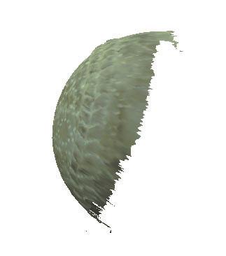
11 2 2.5D 3 2.5D 2.1 ( 2.1(a)) ( 2.1(b)) 2.1: 3
![2 2.5D 2.2 2.1(a) Vivid 9i(Konica Minolta[1]) ( 2.2) 2.](/docs-images/91/105321754/images/12-0.jpg "2: Vivid 9i Vivid 1m ( 2.3) 2.3 2.5D (z) ( 2.4) 2 2.")
12 2 2.5D (a) Vivid 9i(Konica Minolta[1]) ( 2.2) 2.2: Vivid 9i Vivid 1m ( 2.3) D (z) ( 2.4)


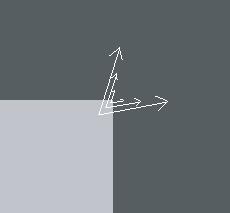
13 D 2.3: 2.4:
14
15 3 2.5D ( ) 3.1 () 2 SIFT[3] SIFT SIFT(Scale Invariant Feature Transform) SIFT

16 3 (detection) (description) 2 ffl ffl ffl ffl 3.1 SIFT 3.1: SIFT SIFT
17 3.1. Difference-of-Gaussian (ff) G(x; y; ff) I(x; y) L(x; y; ff) Difference-of-Gaussian(DoG) L(x; y; ff) =G(x; y; ff) Λ I(x; y) (3.1) G(x; y; ff) = 1 2 +y 2 )=2ff 2 2ßff 2 e (x DoG D(x; y; ff) DoG (3.2) D(x; y; ff) =L(x; y; kff) L(x; y; ff) (3.3) k DoG DoG : Difference-of-Gaussian DoG 3.3 DoG 3 ( ) ( fl ) 9
18 3 3.3: DoG (a) DoG ff 1 3.4(b) DoG ff 2 ff 2 =2ff 1 10
 2 (3.4) x 0 @D @x + @ 2 D ^x =0 (3.")
19 : DoG x =(x; y; ff) T DOG D(x) D(x) =D T x + 2 x (3.4) 2 (3.4) 2 D ^x =0 (3.5) 11
20 3 ^x 2 D ^x 2 (3.) ff y x 3 5 = (3.) (3.) ^x 2 4 ff y x 3 5 = (3.8) (3.8) ^x (3.8) ^x (3.9) (3.4) D(^x) =D + 1 ^x (3.10) ^x 2 H 12
21 3.1. H = 2 4 D xx D xy D xy D yy 3 5 (3.11) 1 ff 2 fi Tr(H) Det(H) Tr(H) = D xx + D yy = ff + fi (3.12) Det(H) = D xx D yy (D xy ) 2 = fffi (3.13) fl 1 2 ff = flfi Tr(H) 2 Det(H) = (ff + fi)2 fffi = (flfi + fi)2 (fl +1)2 = flfi 2 fl (3.14) Tr(H) 2 Det(H) < (fl +1)2 fl (3.15) [3] fl = 10 12: SIFT 2 2.5D 13
22 3 3.1: (12.1) (x; y; z) 3 3.5(a) OAB O OA A OB B A(x 1 ;y 1 ;z 1 )B(x 2 ;y 2 ;z 2 ) A B A B =(y 1 z 2 z 1 y 2 ; z 1 x 2 x 1 z 2 ; x 1 y 2 y 1 x 2 ) (3.1) 14
23 3.2. ( 3.5(b)) 1 N(n 1 ;n 2 ;n 3 ) N ^N = knk = ψ! 1 knk N = n1 n 2 n 3 knk knk knk q (3.1) n n n 2 3 (3.18) ^N 3.5: z ( 3.) 3 15
24 3 3.: 2 4 X 0 Y 0 Z = Tx Ty Tz X Y Z (3.19) Tx;Ty;Tzx y z 2 4 X 0 Y 0 Z = cos sin 0 0 sin cos X Y Z (3.20) 2 4 X 0 Y 0 Z = 2 4 cos 0 sin sin 0 cos X Y Z (3.21) 1
25 X 0 Y 0 Z = 2 4 cos sin 0 0 sin cos X Y Z (3.22) z y x y x 3. ff; fi 3. 3.: N(nx; ny; nz) ff; fi ff = arccos fi = arccos ψ! nz p nx2 + nz 2 ψ p! nx2 + nz p 2 nx2 + ny 2 + nz 2 (3.23) (3.24) 1

 z 2 3.")


26 D ( 3.8) z : 2.5D 18


27 SIFT 3.9: SIFT DoG D 19
28 3 SIFT L(x; y) m(x; y) (x; y) m(x; y) = q (L(x +1;y) L(x 1;y)) 2 +(L(x; y +1) L(x; y 1)) 2 (3.25) (x; y) = tan 1 ((L(x; y +1) L(x; y 1))=(L(x +1;y) L(x 1;y))) (3.2) 3.10 h w(x; y) = G(x; y; ff) m(x; y) (3.2) h = X x X y w(x; y) ffi [ ; (x; y)] (3.28) ffi Kronecker 1.5 h % % 1 2 ( 3.11) ( 3.12) 20
 G(x,")
 3.10:")

29 3.2. w(x, y) G(x, y,) m(x, y) 3.10: 3.11: 2 21
30 3 3.12: : SIFT
31 Shape Index[4] Shape Index Shape Index 0:0 ο 1: Shape Index 3.14: Shape Index 2.5D p Shape Index S(p) k 1 (p);k 2 (p) (k 1 (p) >k 2 (p)) S(p) = ß tan 1 k 1(p)+k 2 (p) k 1 (p) k 2 (p) (3.29) Shape Index p k 1 = k 2 =0 (3.29) 0 0 0:0 ο 1:0 23
32 Shape Index 2.5D p p H = (3.30) x; y; z 2.5D 2 p z (2 ) 2 p z z z Z p (x; y) Z i d i z Z p = P n i=1 P n i=1 Z i d i (3.31) 1 d i z 3.15 Shape Index Shape Index 0 cup 24

33 3.3. Shape Index 1 cap 3.15 Shape Index Shape Index 3.15: Shape Index Shape Index Shape Index 3.2: Shape Index Shape Index ο 0.85 Cap ο Dome ο0.5 Dome ο Ridge ο 0.25 Ridge ο Saddle ridge ο 0.5 Saddle ridge ο Saddle ο 0.35 Saddle ο Saddle rut 0.35 ο 0.25 Saddle rut ο Rut 0.25 ο Rut ο Trough ο 0.0 Trough ο Cup 25
34 3 2
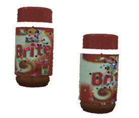
35 D R 1 S R 1 =(s R 1 1 ;sr 1 2 ; ;sr )T R 2 S R 2 =(s R 2 1 ;sr 2 2 ; ;sr )T d(s R 1 ; S R 2 )= X128 i=1 q (s R 1 i s R 2 i ) 2 (4.1) ( 4.1) 2.5D 2
36 4 4.1: 28
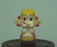
37 5 5.1 Vivid D 2 SIFT 29

![1: [%]](/docs-images/91/105321754/images/38-1.jpg "SIFT 11")


38 % 5.1: [%] SIFT % SIFT 5.1 SIFT : 1 30

![2: [%]](/docs-images/91/105321754/images/39-1.jpg "SIFT 9 5")


39 : [%] SIFT SIFT : SIFT SIFT 31
40
41 2.5D SIFT 33
42
43 35
44
45 [1] Konica Minolta VIVID 9i non-contact 3D laser scanner", [2] Xiaoguang Lu, Dirk Colbry, and Anil K. Jain, Three-Dimensional Model Based Face Recognition," International Conference on Pattern Recognition, (2004), pp [3] D. G. Lowe, Distinctive Image Features from Scale-Invariant Keypoints", International Journal of Computer Vision, 0(2), pp (2004). [4] Chitra Dorai, Anil K. Jain, COSMOS - A Representatin Scheme for 3D Free-Form Objects," IEEE Trans. on PAMI, vol. 19, no. 10, pp ,
46
47 () 200 3
2.2 6).,.,.,. Yang, 7).,,.,,. 2.3 SIFT SIFT (Scale-Invariant Feature Transform) 8).,. SIFT,,. SIFT, Mean-Shift 9)., SIFT,., SIFT,. 3.,.,,,,,.,,,., 1,
.,.,.,. Yang, 7).,,.,,. 2.3 SIFT SIFT (Scale-Invariant Feature Transform) 8).,. SIFT,,. SIFT, Mean-Shift 9)., SIFT,., SIFT,. 3.,.,,,,,.,,,., 1,") 1 1 2,,.,.,,, SIFT.,,. Pitching Motion Analysis Using Image Processing Shinya Kasahara, 1 Issei Fujishiro 1 and Yoshio Ohno 2 At present, analysis of pitching motion from baseball videos is timeconsuming
1 1 2,,.,.,,, SIFT.,,. Pitching Motion Analysis Using Image Processing Shinya Kasahara, 1 Issei Fujishiro 1 and Yoshio Ohno 2 At present, analysis of pitching motion from baseball videos is timeconsuming
 Real AdaBoost HOG 2009 3 A Graduation Thesis of College of Engineering, Chubu University Efficient Reducing Method of HOG Features for Human Detection based on Real AdaBoost Chika Matsushima ITS Graphics
(MIRU2008) HOG Histograms of Oriented Gradients (HOG)
 HOG Histograms of Oriented Gradients (HOG)") (MIRU2008) 2008 7 HOG - - E-mail: katsu0920@me.cs.scitec.kobe-u.ac.jp, {takigu,ariki}@kobe-u.ac.jp Histograms of Oriented Gradients (HOG) HOG Shape Contexts HOG 5.5 Histograms of Oriented Gradients D Human
(MIRU2008) 2008 7 HOG - - E-mail: katsu0920@me.cs.scitec.kobe-u.ac.jp, {takigu,ariki}@kobe-u.ac.jp Histograms of Oriented Gradients (HOG) HOG Shape Contexts HOG 5.5 Histograms of Oriented Gradients D Human
, x R, f (x),, df dx : R R,, f : R R, f(x) ( ).,, f (a) d f dx (a), f (a) d3 f dx 3 (a),, f (n) (a) dn f dx n (a), f d f dx, f d3 f dx 3,, f (n) dn f
,, df dx : R R,, f : R R, f(x) ( ).,, f (a) d f dx (a), f (a) d3 f dx 3 (a),, f (n) (a) dn f dx n (a), f d f dx, f d3 f dx 3,, f (n) dn f") ,,,,.,,,. R f : R R R a R, f(a + ) f(a) lim 0 (), df dx (a) f (a), f(x) x a, f (a), f(x) x a ( ). y f(a + ) y f(x) f(a+) f(a) f(a + ) f(a) f(a) x a 0 a a + x 0 a a + x y y f(x) 0 : 0, f(a+) f(a)., f(x)
,,,,.,,,. R f : R R R a R, f(a + ) f(a) lim 0 (), df dx (a) f (a), f(x) x a, f (a), f(x) x a ( ). y f(a + ) y f(x) f(a+) f(a) f(a + ) f(a) f(a) x a 0 a a + x 0 a a + x y y f(x) 0 : 0, f(a+) f(a)., f(x)
SICE東北支部研究集会資料(2013年)
") 280 (2013.5.29) 280-4 SURF A Study of SURF Algorithm using Edge Image and Color Information Yoshihiro Sasaki, Syunichi Konno, Yoshitaka Tsunekawa * *Iwate University : SURF (Speeded Up Robust Features)
280 (2013.5.29) 280-4 SURF A Study of SURF Algorithm using Edge Image and Color Information Yoshihiro Sasaki, Syunichi Konno, Yoshitaka Tsunekawa * *Iwate University : SURF (Speeded Up Robust Features)
Convolutional Neural Network A Graduation Thesis of College of Engineering, Chubu University Investigation of feature extraction by Convolution
 Convolutional Neural Network 2014 3 A Graduation Thesis of College of Engineering, Chubu University Investigation of feature extraction by Convolutional Neural Network Fukui Hiroshi 1940 1980 [1] 90 3
x = a 1 f (a r, a + r) f(a) r a f f(a) 2 2. (a, b) 2 f (a, b) r f(a, b) r (a, b) f f(a, b)
 f(a) r a f f(a) 2 2. (a, b) 2 f (a, b) r f(a, b) r (a, b) f f(a, b)") 2011 I 2 II III 17, 18, 19 7 7 1 2 2 2 1 2 1 1 1.1.............................. 2 1.2 : 1.................... 4 1.2.1 2............................... 5 1.3 : 2.................... 5 1.3.1 2.....................................
2011 I 2 II III 17, 18, 19 7 7 1 2 2 2 1 2 1 1 1.1.............................. 2 1.2 : 1.................... 4 1.2.1 2............................... 5 1.3 : 2.................... 5 1.3.1 2.....................................
paper.dvi
 23 Study on character extraction from a picture using a gradient-based feature 1120227 2012 3 1 Google Street View Google Street View SIFT 3 SIFT 3 y -80 80-50 30 SIFT i Abstract Study on character extraction
DVIOUT
 A. A. A-- [ ] f(x) x = f 00 (x) f 0 () =0 f 00 () > 0= f(x) x = f 00 () < 0= f(x) x = A--2 [ ] f(x) D f 00 (x) > 0= y = f(x) f 00 (x) < 0= y = f(x) P (, f()) f 00 () =0 A--3 [ ] y = f(x) [, b] x = f (y)
function2.pdf
 2... 1 2009, http://c-faculty.chuo-u.ac.jp/ nishioka/ 2 11 38 : 5) i) [], : 84 85 86 87 88 89 1000 ) 13 22 33 56 92 147 140 120 100 80 60 40 20 1 2 3 4 5 7.1 7 7.1 1. *1 e = 2.7182 ) fx) e x, x R : 7.1)
A Graduation Thesis of College of Engineering, Chubu University Pose Estimation by Regression Analysis with Depth Information Yoshiki Agata
 2011 3 A Graduation Thesis of College of Engineering, Chubu University Pose Estimation by Regression Analysis with Depth Information Yoshiki Agata CG [2] [3][4] 3 3 [1] HOG HOG TOF(Time Of Flight) iii
4 4 4 a b c d a b A c d A a da ad bce O E O n A n O ad bc a d n A n O 5 {a n } S n a k n a n + k S n a a n+ S n n S n n log x x {xy } x, y x + y 7 fx
 4 4 5 4 I II III A B C, 5 7 I II A B,, 8, 9 I II A B O A,, Bb, b, Cc, c, c b c b b c c c OA BC P BC OP BC P AP BC n f n x xn e x! e n! n f n x f n x f n x f k x k 4 e > f n x dx k k! fx sin x cos x tan
x () g(x) = f(t) dt f(x), F (x) 3x () g(x) g (x) f(x), F (x) (3) h(x) = x 3x tf(t) dt.9 = {(x, y) ; x, y, x + y } f(x, y) = xy( x y). h (x) f(x), F (x
 g(x) = f(t) dt f(x), F (x) 3x () g(x) g (x) f(x), F (x) (3) h(x) = x 3x tf(t) dt.9 = {(x, y) ; x, y, x + y } f(x, y) = xy( x y). h (x) f(x), F (x") [ ] IC. f(x) = e x () f(x) f (x) () lim f(x) lim f(x) x + x (3) lim f(x) lim f(x) x + x (4) y = f(x) ( ) ( s46). < a < () a () lim a log xdx a log xdx ( ) n (3) lim log k log n n n k=.3 z = log(x + y ),
[ ] IC. f(x) = e x () f(x) f (x) () lim f(x) lim f(x) x + x (3) lim f(x) lim f(x) x + x (4) y = f(x) ( ) ( s46). < a < () a () lim a log xdx a log xdx ( ) n (3) lim log k log n n n k=.3 z = log(x + y ),
paper.dvi
 SIFT 23 (410M5B1) SIFT(Scale Invariant Feature Transform) SIFT SIFT SIFT SIMD SIFT SIMD MIMD Gaussian SIMD Abstract Currently, with the development of image-recognition technique, to recognize a large
1: *2 W, L 2 1 (WWL) 4 5 (WWL) W (WWL) L W (WWL) L L 1 2, 1 4, , 1 4 (cf. [4]) 2: 2 3 * , , = , 1
![1: *2 W, L 2 1 (WWL) 4 5 (WWL) W (WWL) L W (WWL) L L 1 2, 1 4, , 1 4 (cf. [4]) 2: 2 3 * , , = , 1](/thumbs/49/25412084.jpg "1: *2 W, L 2 1 (WWL) 4 5 (WWL) W (WWL) L W (WWL) L L 1 2, 1 4, , 1 4 (cf. [4]) 2: 2 3 * , , = , 1") I, A 25 8 24 1 1.1 ( 3 ) 3 9 10 3 9 : (1,2,6), (1,3,5), (1,4,4), (2,2,5), (2,3,4), (3,3,3) 10 : (1,3,6), (1,4,5), (2,2,6), (2,3,5), (2,4,4), (3,3,4) 6 3 9 10 3 9 : 6 3 + 3 2 + 1 = 25 25 10 : 6 3 + 3 3
I, A 25 8 24 1 1.1 ( 3 ) 3 9 10 3 9 : (1,2,6), (1,3,5), (1,4,4), (2,2,5), (2,3,4), (3,3,3) 10 : (1,3,6), (1,4,5), (2,2,6), (2,3,5), (2,4,4), (3,3,4) 6 3 9 10 3 9 : 6 3 + 3 2 + 1 = 25 25 10 : 6 3 + 3 3
di-problem.dvi
 2005/04/4 by. : : : : : : : : : : : : : : : : : : : : : : : : : : 2 2. : : : : : : : : : : : : : : : : : : : : : : 3 3. : : : : : : : : : : : : : : : : : : : : : : : : : 4 4. : : : : : : : : : : : : :
i
 i 3 4 4 7 5 6 3 ( ).. () 3 () (3) (4) /. 3. 4/3 7. /e 8. a > a, a = /, > a >. () a >, a =, > a > () a > b, a = b, a < b. c c n a n + b n + c n 3c n..... () /3 () + (3) / (4) /4 (5) m > n, a b >, m > n,
ax 2 + bx + c = n 8 (n ) a n x n + a n 1 x n a 1 x + a 0 = 0 ( a n, a n 1,, a 1, a 0 a n 0) n n ( ) ( ) ax 3 + bx 2 + cx + d = 0 4
 a n x n + a n 1 x n a 1 x + a 0 = 0 ( a n, a n 1,, a 1, a 0 a n 0) n n ( ) ( ) ax 3 + bx 2 + cx + d = 0 4") 20 20.0 ( ) 8 y = ax 2 + bx + c 443 ax 2 + bx + c = 0 20.1 20.1.1 n 8 (n ) a n x n + a n 1 x n 1 + + a 1 x + a 0 = 0 ( a n, a n 1,, a 1, a 0 a n 0) n n ( ) ( ) ax 3 + bx 2 + cx + d = 0 444 ( a, b, c, d
20 20.0 ( ) 8 y = ax 2 + bx + c 443 ax 2 + bx + c = 0 20.1 20.1.1 n 8 (n ) a n x n + a n 1 x n 1 + + a 1 x + a 0 = 0 ( a n, a n 1,, a 1, a 0 a n 0) n n ( ) ( ) ax 3 + bx 2 + cx + d = 0 444 ( a, b, c, d
SAR: Synthetic Aperture Radar 0.52 Radarsat SAR 2004 ALOS i
 2002 Noise Reduction and Application of Ocean Images Using Synthetic Aperture Radar Slide-Look Processing 2003 2 21 1055147 SAR: Synthetic Aperture Radar 0.52 Radarsat SAR 2004 ALOS i 1 1 1.1 : : : : :
Duplicate Near Duplicate Intact Partial Copy Original Image Near Partial Copy Near Partial Copy with a background (a) (b) 2 1 [6] SIFT SIFT SIF
![Duplicate Near Duplicate Intact Partial Copy Original Image Near Partial Copy Near Partial Copy with a background (a) (b) 2 1 [6] SIFT SIFT SIF](/thumbs/82/86406952.jpg "Duplicate Near Duplicate Intact Partial Copy Original Image Near Partial Copy Near Partial Copy with a background (a) (b) 2 1 [6] SIFT SIFT SIF") Partial Copy Detection of Line Drawings from a Large-Scale Database Weihan Sun, Koichi Kise Graduate School of Engineering, Osaka Prefecture University E-mail: sunweihan@m.cs.osakafu-u.ac.jp, kise@cs.osakafu-u.ac.jp
Partial Copy Detection of Line Drawings from a Large-Scale Database Weihan Sun, Koichi Kise Graduate School of Engineering, Osaka Prefecture University E-mail: sunweihan@m.cs.osakafu-u.ac.jp, kise@cs.osakafu-u.ac.jp
II Karel Švadlenka * [1] 1.1* 5 23 m d2 x dt 2 = cdx kx + mg dt. c, g, k, m 1.2* u = au + bv v = cu + dv v u a, b, c, d R
![II Karel Švadlenka * [1] 1.1* 5 23 m d2 x dt 2 = cdx kx + mg dt. c, g, k, m 1.2* u = au + bv v = cu + dv v u a, b, c, d R](/thumbs/95/125540821.jpg "II Karel Švadlenka * [1] 1.1* 5 23 m d2 x dt 2 = cdx kx + mg dt. c, g, k, m 1.2* u = au + bv v = cu + dv v u a, b, c, d R") II Karel Švadlenka 2018 5 26 * [1] 1.1* 5 23 m d2 x dt 2 = cdx kx + mg dt. c, g, k, m 1.2* 5 23 1 u = au + bv v = cu + dv v u a, b, c, d R 1.3 14 14 60% 1.4 5 23 a, b R a 2 4b < 0 λ 2 + aλ + b = 0 λ =
II Karel Švadlenka 2018 5 26 * [1] 1.1* 5 23 m d2 x dt 2 = cdx kx + mg dt. c, g, k, m 1.2* 5 23 1 u = au + bv v = cu + dv v u a, b, c, d R 1.3 14 14 60% 1.4 5 23 a, b R a 2 4b < 0 λ 2 + aλ + b = 0 λ =
di-problem.dvi
 005/05/05 by. I : : : : : : : : : : : : : : : : : : : : : : : : :. II : : : : : : : : : : : : : : : : : : : : : : : : : 3 3. III : : : : : : : : : : : : : : : : : : : : : : : : 4 4. : : : : : : : : : :
S I. dy fx x fx y fx + C 3 C vt dy fx 4 x, y dy yt gt + Ct + C dt v e kt xt v e kt + C k x v k + C C xt v k 3 r r + dr e kt S Sr πr dt d v } dt k e kt
 S I. x yx y y, y,. F x, y, y, y,, y n http://ayapin.film.s.dendai.ac.jp/~matuda n /TeX/lecture.html PDF PS yx.................................... 3.3.................... 9.4................5..............
% 2 3 [1] Semantic Texton Forests STFs [1] ( ) STFs STFs ColorSelf-Simlarity CSS [2] ii
![% 2 3 [1] Semantic Texton Forests STFs [1] ( ) STFs STFs ColorSelf-Simlarity CSS [2] ii](/thumbs/91/106152959.jpg "% 2 3 [1] Semantic Texton Forests STFs [1] ( ) STFs STFs ColorSelf-Simlarity CSS [2] ii") 2012 3 A Graduation Thesis of College of Engineering, Chubu University High Accurate Semantic Segmentation Using Re-labeling Besed on Color Self Similarity Yuko KAKIMI 2400 90% 2 3 [1] Semantic Texton
2012 3 A Graduation Thesis of College of Engineering, Chubu University High Accurate Semantic Segmentation Using Re-labeling Besed on Color Self Similarity Yuko KAKIMI 2400 90% 2 3 [1] Semantic Texton
 211 kotaro@math.titech.ac.jp 1 R *1 n n R n *2 R n = {(x 1,..., x n ) x 1,..., x n R}. R R 2 R 3 R n R n R n D D R n *3 ) (x 1,..., x n ) f(x 1,..., x n ) f D *4 n 2 n = 1 ( ) 1 f D R n f : D R 1.1. (x,
t = h x z z = h z = t (x, z) (v x (x, z, t), v z (x, z, t)) ρ v x x + v z z = 0 (1) 2-2. (v x, v z ) φ(x, z, t) v x = φ x, v z
 (v x (x, z, t), v z (x, z, t)) ρ v x x + v z z = 0 (1) 2-2. (v x, v z ) φ(x, z, t) v x = φ x, v z") I 1 m 2 l k 2 x = 0 x 1 x 1 2 x 2 g x x 2 x 1 m k m 1-1. L x 1, x 2, ẋ 1, ẋ 2 ẋ 1 x = 0 1-2. 2 Q = x 1 + x 2 2 q = x 2 x 1 l L Q, q, Q, q M = 2m µ = m 2 1-3. Q q 1-4. 2 x 2 = h 1 x 1 t = 0 2 1 t x 1 (t)
I 1 m 2 l k 2 x = 0 x 1 x 1 2 x 2 g x x 2 x 1 m k m 1-1. L x 1, x 2, ẋ 1, ẋ 2 ẋ 1 x = 0 1-2. 2 Q = x 1 + x 2 2 q = x 2 x 1 l L Q, q, Q, q M = 2m µ = m 2 1-3. Q q 1-4. 2 x 2 = h 1 x 1 t = 0 2 1 t x 1 (t)
No2 4 y =sinx (5) y = p sin(2x +3) (6) y = 1 tan(3x 2) (7) y =cos 2 (4x +5) (8) y = cos x 1+sinx 5 (1) y =sinx cos x 6 f(x) = sin(sin x) f 0 (π) (2) y
 y = p sin(2x +3) (6) y = 1 tan(3x 2) (7) y =cos 2 (4x +5) (8) y = cos x 1+sinx 5 (1) y =sinx cos x 6 f(x) = sin(sin x) f 0 (π) (2) y") No1 1 (1) 2 f(x) =1+x + x 2 + + x n, g(x) = 1 (n +1)xn + nx n+1 (1 x) 2 x 6= 1 f 0 (x) =g(x) y = f(x)g(x) y 0 = f 0 (x)g(x)+f(x)g 0 (x) 3 (1) y = x2 x +1 x (2) y = 1 g(x) y0 = g0 (x) {g(x)} 2 (2) y = µ
No1 1 (1) 2 f(x) =1+x + x 2 + + x n, g(x) = 1 (n +1)xn + nx n+1 (1 x) 2 x 6= 1 f 0 (x) =g(x) y = f(x)g(x) y 0 = f 0 (x)g(x)+f(x)g 0 (x) 3 (1) y = x2 x +1 x (2) y = 1 g(x) y0 = g0 (x) {g(x)} 2 (2) y = µ
[1] SBS [2] SBS Random Forests[3] Random Forests ii
![[1] SBS [2] SBS Random Forests[3] Random Forests ii](/thumbs/74/70333192.jpg "[1] SBS [2] SBS Random Forests[3] Random Forests ii") Random Forests 2013 3 A Graduation Thesis of College of Engineering, Chubu University Proposal of an efficient feature selection using the contribution rate of Random Forests Katsuya Shimazaki [1] SBS
Random Forests 2013 3 A Graduation Thesis of College of Engineering, Chubu University Proposal of an efficient feature selection using the contribution rate of Random Forests Katsuya Shimazaki [1] SBS
IPSJ SIG Technical Report Vol.2010-CVIM-170 No /1/ Visual Recognition of Wire Harnesses for Automated Wiring Masaki Yoneda, 1 Ta
 1 1 1 1 2 1. Visual Recognition of Wire Harnesses for Automated Wiring Masaki Yoneda, 1 Takayuki Okatani 1 and Koichiro Deguchi 1 This paper presents a method for recognizing the pose of a wire harness
6kg 1.1m 1.m.1m.1 l λ ϵ λ l + λ l l l dl dl + dλ ϵ dλ dl dl + dλ dl dl 3 1. JIS 1 6kg 1% 66kg 1 13 σ a1 σ m σ a1 σ m σ m σ a1 f f σ a1 σ a1 σ m f 4
 35-8585 7 8 1 I I 1 1.1 6kg 1m P σ σ P 1 l l λ λ l 1.m 1 6kg 1.1m 1.m.1m.1 l λ ϵ λ l + λ l l l dl dl + dλ ϵ dλ dl dl + dλ dl dl 3 1. JIS 1 6kg 1% 66kg 1 13 σ a1 σ m σ a1 σ m σ m σ a1 f f σ a1 σ a1 σ m
5. [1 ] 1 [], u(x, t) t c u(x, t) x (5.3) ξ x + ct, η x ct (5.4),u(x, t) ξ, η u(ξ, η), ξ t,, ( u(ξ,η) ξ η u(x, t) t ) u(x, t) { ( u(ξ, η) c t ξ ξ { (
![5. [1 ] 1 [], u(x, t) t c u(x, t) x (5.3) ξ x + ct, η x ct (5.4),u(x, t) ξ, η u(ξ, η), ξ t,, ( u(ξ,η) ξ η u(x, t) t ) u(x, t) { ( u(ξ, η) c t ξ ξ { (](/thumbs/92/107866626.jpg "5. [1 ] 1 [], u(x, t) t c u(x, t) x (5.3) ξ x + ct, η x ct (5.4),u(x, t) ξ, η u(ξ, η), ξ t,, ( u(ξ,η) ξ η u(x, t) t ) u(x, t) { ( u(ξ, η) c t ξ ξ { (") 5 5.1 [ ] ) d f(t) + a d f(t) + bf(t) : f(t) 1 dt dt ) u(x, t) c u(x, t) : u(x, t) t x : ( ) ) 1 : y + ay, : y + ay + by : ( ) 1 ) : y + ay, : yy + ay 3 ( ): ( ) ) : y + ay, : y + ay b [],,, [ ] au xx
5 5.1 [ ] ) d f(t) + a d f(t) + bf(t) : f(t) 1 dt dt ) u(x, t) c u(x, t) : u(x, t) t x : ( ) ) 1 : y + ay, : y + ay + by : ( ) 1 ) : y + ay, : yy + ay 3 ( ): ( ) ) : y + ay, : y + ay b [],,, [ ] au xx
6. Euler x
 ...............................................................................3......................................... 4.4................................... 5.5......................................
S I. dy fx x fx y fx + C 3 C dy fx 4 x, y dy v C xt y C v e kt k > xt yt gt [ v dt dt v e kt xt v e kt + C k x v + C C k xt v k 3 r r + dr e kt S dt d
 S I.. http://ayapin.film.s.dendai.ac.jp/~matuda /TeX/lecture.html PDF PS.................................... 3.3.................... 9.4................5.............. 3 5. Laplace................. 5....
熊本県数学問題正解
 00 y O x Typed by L A TEX ε ( ) (00 ) 5 4 4 ( ) http://www.ocn.ne.jp/ oboetene/plan/. ( ) (009 ) ( ).. http://www.ocn.ne.jp/ oboetene/plan/eng.html 8 i i..................................... ( )0... (


() n C + n C + n C + + n C n n (3) n C + n C + n C 4 + n C + n C 3 + n C 5 + (5) (6 ) n C + nc + 3 nc n nc n (7 ) n C + nc + 3 nc n nc n (
 n C + n C + n C + + n C n n (3) n C + n C + n C 4 + n C + n C 3 + n C 5 + (5) (6 ) n C + nc + 3 nc n nc n (7 ) n C + nc + 3 nc n nc n (") 3 n nc k+ k + 3 () n C r n C n r nc r C r + C r ( r n ) () n C + n C + n C + + n C n n (3) n C + n C + n C 4 + n C + n C 3 + n C 5 + (4) n C n n C + n C + n C + + n C n (5) k k n C k n C k (6) n C + nc
3 n nc k+ k + 3 () n C r n C n r nc r C r + C r ( r n ) () n C + n C + n C + + n C n n (3) n C + n C + n C 4 + n C + n C 3 + n C 5 + (4) n C n n C + n C + n C + + n C n (5) k k n C k n C k (6) n C + nc
W u = u(x, t) u tt = a 2 u xx, a > 0 (1) D := {(x, t) : 0 x l, t 0} u (0, t) = 0, u (l, t) = 0, t 0 (2)
 u tt = a 2 u xx, a > 0 (1) D := {(x, t) : 0 x l, t 0} u (0, t) = 0, u (l, t) = 0, t 0 (2)") 3 215 4 27 1 1 u u(x, t) u tt a 2 u xx, a > (1) D : {(x, t) : x, t } u (, t), u (, t), t (2) u(x, ) f(x), u(x, ) t 2, x (3) u(x, t) X(x)T (t) u (1) 1 T (t) a 2 T (t) X (x) X(x) α (2) T (t) αa 2 T (t) (4)
3 215 4 27 1 1 u u(x, t) u tt a 2 u xx, a > (1) D : {(x, t) : x, t } u (, t), u (, t), t (2) u(x, ) f(x), u(x, ) t 2, x (3) u(x, t) X(x)T (t) u (1) 1 T (t) a 2 T (t) X (x) X(x) α (2) T (t) αa 2 T (t) (4)
Part y mx + n mt + n m 1 mt n + n t m 2 t + mn 0 t m 0 n 18 y n n a 7 3 ; x α α 1 7α +t t 3 4α + 3t t x α x α y mx + n
 Part2 47 Example 161 93 1 T a a 2 M 1 a 1 T a 2 a Point 1 T L L L T T L L T L L L T T L L T detm a 1 aa 2 a 1 2 + 1 > 0 11 T T x x M λ 12 y y x y λ 2 a + 1λ + a 2 2a + 2 0 13 D D a + 1 2 4a 2 2a + 2 a
28 Horizontal angle correction using straight line detection in an equirectangular image
 28 Horizontal angle correction using straight line detection in an equirectangular image 1170283 2017 3 1 2 i Abstract Horizontal angle correction using straight line detection in an equirectangular image
微分積分 サンプルページ この本の定価 判型などは, 以下の URL からご覧いただけます. このサンプルページの内容は, 初版 1 刷発行時のものです.
 微分積分 サンプルページ この本の定価 判型などは, 以下の URL からご覧いただけます. ttp://www.morikita.co.jp/books/mid/00571 このサンプルページの内容は, 初版 1 刷発行時のものです. i ii 014 10 iii [note] 1 3 iv 4 5 3 6 4 x 0 sin x x 1 5 6 z = f(x, y) 1 y = f(x)
x (x, ) x y (, y) iy x y z = x + iy (x, y) (r, θ) r = x + y, θ = tan ( y ), π < θ π x r = z, θ = arg z z = x + iy = r cos θ + ir sin θ = r(cos θ + i s
 x y (, y) iy x y z = x + iy (x, y) (r, θ) r = x + y, θ = tan ( y ), π < θ π x r = z, θ = arg z z = x + iy = r cos θ + ir sin θ = r(cos θ + i s") ... x, y z = x + iy x z y z x = Rez, y = Imz z = x + iy x iy z z () z + z = (z + z )() z z = (z z )(3) z z = ( z z )(4)z z = z z = x + y z = x + iy ()Rez = (z + z), Imz = (z z) i () z z z + z z + z.. z
... x, y z = x + iy x z y z x = Rez, y = Imz z = x + iy x iy z z () z + z = (z + z )() z z = (z z )(3) z z = ( z z )(4)z z = z z = x + y z = x + iy ()Rez = (z + z), Imz = (z z) i () z z z + z z + z.. z
IPSJ SIG Technical Report Vol.2012-CG-149 No.13 Vol.2012-CVIM-184 No /12/4 3 1,a) ( ) DB 3D DB 2D,,,, PnP(Perspective n-point), Ransa
 ( ) DB 3D DB 2D,,,, PnP(Perspective n-point), Ransa") 3,a) 3 3 ( ) DB 3D DB 2D,,,, PnP(Perspective n-point), Ransac. DB [] [2] 3 DB Web Web DB Web NTT NTT Media Intelligence Laboratories, - Hikarinooka Yokosuka-Shi, Kanagawa 239-0847 Japan a) yabushita.hiroko@lab.ntt.co.jp
3,a) 3 3 ( ) DB 3D DB 2D,,,, PnP(Perspective n-point), Ransac. DB [] [2] 3 DB Web Web DB Web NTT NTT Media Intelligence Laboratories, - Hikarinooka Yokosuka-Shi, Kanagawa 239-0847 Japan a) yabushita.hiroko@lab.ntt.co.jp
入試の軌跡
 4 y O x 4 Typed by L A TEX ε ) ) ) 6 4 ) 4 75 ) http://kumamoto.s.xrea.com/plan/.. PDF) Ctrl +L) Ctrl +) Ctrl + Ctrl + ) ) Alt + ) Alt + ) ESC. http://kumamoto.s.xrea.com/nyusi/kumadai kiseki ri i.pdf
A A = a 41 a 42 a 43 a 44 A (7) 1 (3) A = M 12 = = a 41 (8) a 41 a 43 a 44 (3) n n A, B a i AB = A B ii aa
 1 (3) A = M 12 = = a 41 (8) a 41 a 43 a 44 (3) n n A, B a i AB = A B ii aa") 1 2 21 2 2 [ ] a 11 a 12 A = a 21 a 22 (1) A = a 11 a 22 a 12 a 21 (2) 3 3 n n A A = n ( 1) i+j a ij M ij i =1 n (3) j=1 M ij A i j (n 1) (n 1) 2-1 3 3 A A = a 11 a 12 a 13 a 21 a 22 a 23 a 31 a 32 a 33
1 2 21 2 2 [ ] a 11 a 12 A = a 21 a 22 (1) A = a 11 a 22 a 12 a 21 (2) 3 3 n n A A = n ( 1) i+j a ij M ij i =1 n (3) j=1 M ij A i j (n 1) (n 1) 2-1 3 3 A A = a 11 a 12 a 13 a 21 a 22 a 23 a 31 a 32 a 33
2009 IA 5 I 22, 23, 24, 25, 26, (1) Arcsin 1 ( 2 (4) Arccos 1 ) 2 3 (2) Arcsin( 1) (3) Arccos 2 (5) Arctan 1 (6) Arctan ( 3 ) 3 2. n (1) ta
 Arcsin 1 ( 2 (4) Arccos 1 ) 2 3 (2) Arcsin( 1) (3) Arccos 2 (5) Arctan 1 (6) Arctan ( 3 ) 3 2. n (1) ta") 009 IA 5 I, 3, 4, 5, 6, 7 6 3. () Arcsin ( (4) Arccos ) 3 () Arcsin( ) (3) Arccos (5) Arctan (6) Arctan ( 3 ) 3. n () tan x (nπ π/, nπ + π/) f n (x) f n (x) fn (x) Arctan x () sin x [nπ π/, nπ +π/] g n
009 IA 5 I, 3, 4, 5, 6, 7 6 3. () Arcsin ( (4) Arccos ) 3 () Arcsin( ) (3) Arccos (5) Arctan (6) Arctan ( 3 ) 3. n () tan x (nπ π/, nπ + π/) f n (x) f n (x) fn (x) Arctan x () sin x [nπ π/, nπ +π/] g n
.Z.p...\...X.g
 KONICA MINOLTA TECHNOLOGY REPORT VOL.2 2005 199 7 200 KONICA MINOLTA TECHNOLOGY REPORT VOL.2 2005 KONICA MINOLTA TECHNOLOGY REPORT VOL.2 2005 201 202 KONICA MINOLTA TECHNOLOGY REPORT VOL.2 2005 203 KONICA
.Z.p...\...X.g2007
 108 KONICA MINOLTA TECHNOLOGY REPORT VOL.42007 KONICA MINOLTA TECHNOLOGY REPORT VOL.42007 109 110 KONICA MINOLTA TECHNOLOGY REPORT VOL.42007 8 KONICA MINOLTA TECHNOLOGY REPORT VOL.42007 111 112 KONICA
IPSJ SIG Technical Report iphone iphone,,., OpenGl ES 2.0 GLSL(OpenGL Shading Language), iphone GPGPU(General-Purpose Computing on Graphics Proc
, iphone GPGPU(General-Purpose Computing on Graphics Proc") iphone 1 1 1 iphone,,., OpenGl ES 2.0 GLSL(OpenGL Shading Language), iphone GPGPU(General-Purpose Computing on Graphics Processing Unit)., AR Realtime Natural Feature Tracking Library for iphone Makoto
iphone 1 1 1 iphone,,., OpenGl ES 2.0 GLSL(OpenGL Shading Language), iphone GPGPU(General-Purpose Computing on Graphics Processing Unit)., AR Realtime Natural Feature Tracking Library for iphone Makoto
1 No.1 5 C 1 I III F 1 F 2 F 1 F 2 2 Φ 2 (t) = Φ 1 (t) Φ 1 (t t). = Φ 1(t) t = ( 1.5e 0.5t 2.4e 4t 2e 10t ) τ < 0 t > τ Φ 2 (t) < 0 lim t Φ 2 (t) = 0
 = Φ 1 (t) Φ 1 (t t). = Φ 1(t) t = ( 1.5e 0.5t 2.4e 4t 2e 10t ) τ < 0 t > τ Φ 2 (t) < 0 lim t Φ 2 (t) = 0") 1 No.1 5 C 1 I III F 1 F 2 F 1 F 2 2 Φ 2 (t) = Φ 1 (t) Φ 1 (t t). = Φ 1(t) t = ( 1.5e 0.5t 2.4e 4t 2e 10t ) τ < 0 t > τ Φ 2 (t) < 0 lim t Φ 2 (t) = 0 0 < t < τ I II 0 No.2 2 C x y x y > 0 x 0 x > b a dx
1 No.1 5 C 1 I III F 1 F 2 F 1 F 2 2 Φ 2 (t) = Φ 1 (t) Φ 1 (t t). = Φ 1(t) t = ( 1.5e 0.5t 2.4e 4t 2e 10t ) τ < 0 t > τ Φ 2 (t) < 0 lim t Φ 2 (t) = 0 0 < t < τ I II 0 No.2 2 C x y x y > 0 x 0 x > b a dx
情報処理学会研究報告 IPSJ SIG Technical Report Vol.2013-CVIM-186 No /3/15 EMD 1,a) SIFT. SIFT Bag-of-keypoints. SIFT SIFT.. Earth Mover s Distance
 SIFT. SIFT Bag-of-keypoints. SIFT SIFT.. Earth Mover s Distance") EMD 1,a) 1 1 1 SIFT. SIFT Bag-of-keypoints. SIFT SIFT.. Earth Mover s Distance (EMD), Bag-of-keypoints,. Bag-of-keypoints, SIFT, EMD, A method of similar image retrieval system using EMD and SIFT Hoshiga
EMD 1,a) 1 1 1 SIFT. SIFT Bag-of-keypoints. SIFT SIFT.. Earth Mover s Distance (EMD), Bag-of-keypoints,. Bag-of-keypoints, SIFT, EMD, A method of similar image retrieval system using EMD and SIFT Hoshiga
Optical Flow t t + δt 1 Motion Field 3 3 1) 2) 3) Lucas-Kanade 4) 1 t (x, y) I(x, y, t)
 2) 3) Lucas-Kanade 4) 1 t (x, y) I(x, y, t)") http://wwwieice-hbkborg/ 2 2 4 2 -- 2 4 2010 9 3 3 4-1 Lucas-Kanade 4-2 Mean Shift 3 4-3 2 c 2013 1/(18) http://wwwieice-hbkborg/ 2 2 4 2 -- 2 -- 4 4--1 2010 9 4--1--1 Optical Flow t t + δt 1 Motion Field
http://wwwieice-hbkborg/ 2 2 4 2 -- 2 4 2010 9 3 3 4-1 Lucas-Kanade 4-2 Mean Shift 3 4-3 2 c 2013 1/(18) http://wwwieice-hbkborg/ 2 2 4 2 -- 2 -- 4 4--1 2010 9 4--1--1 Optical Flow t t + δt 1 Motion Field
III
 III 1 1 2 1 2 3 1 3 4 1 3 1 4 1 3 2 4 1 3 3 6 1 4 6 1 4 1 6 1 4 2 8 1 4 3 9 1 5 10 1 5 1 10 1 5 2 12 1 5 3 12 1 5 4 13 1 6 15 2 1 18 2 1 1 18 2 1 2 19 2 2 20 2 3 22 2 3 1 22 2 3 2 24 2 4 25 2 4 1 25 2
 iii iv v vi vii viii ix 1 1-1 1-2 1-3 2 2-1 3 3-1 3-2 3-3 3-4 4 4-1 4-2 5 5-1 5-2 5-3 5-4 5-5 5-6 5-7 6 6-1 6-2 6-3 6-4 6-5 6 6-1 6-2 6-3 6-4 6-5 7 7-1 7-2 7-3 7-4 7-5 7-6 7-7 7-8 7-9 7-10 7-11 8 8-1
スライド 1
 (version 2011/9/27) 2 1 H i 1 1 2 5 21 : : : : : : : : : : : : : : : : : : : : : : : : : : : : : : : : : : : : 5 22 : : : : : : : : : : : : : : : : : : : : : : : : : : : : : : : 5 23 : : : : : : : : :
1
 1 1 7 1.1.................................. 11 2 13 2.1............................ 13 2.2............................ 17 2.3.................................. 19 3 21 3.1.............................
LBP 2 LBP 2. 2 Local Binary Pattern Local Binary pattern(lbp) [6] R
![LBP 2 LBP 2. 2 Local Binary Pattern Local Binary pattern(lbp) [6] R](/thumbs/86/93333816.jpg "LBP 2 LBP 2. 2 Local Binary Pattern Local Binary pattern(lbp) [6] R") DEIM Forum 24 F5-4 Local Binary Pattern 6 84 E-mail: {tera,kida}@ist.hokudai.ac.jp Local Binary Pattern (LBP) LBP 3 3 LBP 5 5 5 LBP improved LBP uniform LBP.. Local Binary Pattern, Gradient Local Auto-Correlations,,,,
DEIM Forum 24 F5-4 Local Binary Pattern 6 84 E-mail: {tera,kida}@ist.hokudai.ac.jp Local Binary Pattern (LBP) LBP 3 3 LBP 5 5 5 LBP improved LBP uniform LBP.. Local Binary Pattern, Gradient Local Auto-Correlations,,,,
1 yousuke.itoh/lecture-notes.html [0, π) f(x) = x π 2. [0, π) f(x) = x 2π 3. [0, π) f(x) = x 2π 1.2. Euler α
 f(x) = x π 2. [0, π) f(x) = x 2π 3. [0, π) f(x) = x 2π 1.2. Euler α") 1 http://sasuke.hep.osaka-cu.ac.jp/ yousuke.itoh/lecture-notes.html 1.1. 1. [, π) f(x) = x π 2. [, π) f(x) = x 2π 3. [, π) f(x) = x 2π 1.2. Euler dx = 2π, cos mxdx =, sin mxdx =, cos nx cos mxdx = πδ mn,
1 http://sasuke.hep.osaka-cu.ac.jp/ yousuke.itoh/lecture-notes.html 1.1. 1. [, π) f(x) = x π 2. [, π) f(x) = x 2π 3. [, π) f(x) = x 2π 1.2. Euler dx = 2π, cos mxdx =, sin mxdx =, cos nx cos mxdx = πδ mn,
2 7 V 7 {fx fx 3 } 8 P 3 {fx fx 3 } 9 V 9 {fx fx f x 2fx } V {fx fx f x 2fx + } V {{a n } {a n } a n+2 a n+ + a n n } 2 V 2 {{a n } {a n } a n+2 a n+
 R 3 R n C n V??,?? k, l K x, y, z K n, i x + y + z x + y + z iv x V, x + x o x V v kx + y kx + ky vi k + lx kx + lx vii klx klx viii x x ii x + y y + x, V iii o K n, x K n, x + o x iv x K n, x + x o x
(a) (b) (c) Canny (d) 1 ( x α, y α ) 3 (x α, y α ) (a) A 2 + B 2 + C 2 + D 2 + E 2 + F 2 = 1 (3) u ξ α u (A, B, C, D, E, F ) (4) ξ α (x 2 α, 2x α y α,
 (b) (c) Canny (d) 1 ( x α, y α ) 3 (x α, y α ) (a) A 2 + B 2 + C 2 + D 2 + E 2 + F 2 = 1 (3) u ξ α u (A, B, C, D, E, F ) (4) ξ α (x 2 α, 2x α y α,") [II] Optimization Computation for 3-D Understanding of Images [II]: Ellipse Fitting 1. (1) 2. (2) (edge detection) (edge) (zero-crossing) Canny (Canny operator) (3) 1(a) [I] [II] [III] [IV ] E-mail sugaya@iim.ics.tut.ac.jp
[II] Optimization Computation for 3-D Understanding of Images [II]: Ellipse Fitting 1. (1) 2. (2) (edge detection) (edge) (zero-crossing) Canny (Canny operator) (3) 1(a) [I] [II] [III] [IV ] E-mail sugaya@iim.ics.tut.ac.jp
X線-m.dvi
 X Λ 1 X 1 O Y Z X Z ν X O r Y ' P I('; r) =I e 4 m c 4 1 r sin ' (1.1) I X 1sec 1cm e = 4:8 1 1 e.s.u. m = :1 1 8 g c =3: 1 1 cm/sec X sin '! 1 ß Z ß Z sin 'd! = 1 ß ß 1 sin χ cos! d! = 1+cos χ (1.) e
18 ( ) I II III A B C(100 ) 1, 2, 3, 5 I II A B (100 ) 1, 2, 3 I II A B (80 ) 6 8 I II III A B C(80 ) 1 n (1 + x) n (1) n C 1 + n C
 I II III A B C(100 ) 1, 2, 3, 5 I II A B (100 ) 1, 2, 3 I II A B (80 ) 6 8 I II III A B C(80 ) 1 n (1 + x) n (1) n C 1 + n C") 8 ( ) 8 5 4 I II III A B C( ),,, 5 I II A B ( ),, I II A B (8 ) 6 8 I II III A B C(8 ) n ( + x) n () n C + n C + + n C n = 7 n () 7 9 C : y = x x A(, 6) () A C () C P AP Q () () () 4 A(,, ) B(,, ) C(,,
8 ( ) 8 5 4 I II III A B C( ),,, 5 I II A B ( ),, I II A B (8 ) 6 8 I II III A B C(8 ) n ( + x) n () n C + n C + + n C n = 7 n () 7 9 C : y = x x A(, 6) () A C () C P AP Q () () () 4 A(,, ) B(,, ) C(,,
III No (i) (ii) (iii) (iv) (v) (vi) x 2 3xy + 2 lim. (x,y) (1,0) x 2 + y 2 lim (x,y) (0,0) lim (x,y) (0,0) lim (x,y) (0,0) 5x 2 y x 2 + y 2. xy x2 + y
 (ii) (iii) (iv) (v) (vi) x 2 3xy + 2 lim. (x,y) (1,0) x 2 + y 2 lim (x,y) (0,0) lim (x,y) (0,0) lim (x,y) (0,0) 5x 2 y x 2 + y 2. xy x2 + y") III No (i) (ii) (iii) (iv) (v) (vi) x 2 3xy + 2. (x,y) (1,0) x 2 + y 2 5x 2 y x 2 + y 2. xy x2 + y 2. 2x + y 3 x 2 + y 2 + 5. sin(x 2 + y 2 ). x 2 + y 2 sin(x 2 y + xy 2 ). xy (i) (ii) (iii) 2xy x 2 +
III No (i) (ii) (iii) (iv) (v) (vi) x 2 3xy + 2. (x,y) (1,0) x 2 + y 2 5x 2 y x 2 + y 2. xy x2 + y 2. 2x + y 3 x 2 + y 2 + 5. sin(x 2 + y 2 ). x 2 + y 2 sin(x 2 y + xy 2 ). xy (i) (ii) (iii) 2xy x 2 +
40 6 y mx x, y 0, 0 x 0. x,y 0,0 y x + y x 0 mx x + mx m + m m 7 sin y x, x x sin y x x. x sin y x,y 0,0 x 0. 8 x r cos θ y r sin θ x, y 0, 0, r 0. x,
 9.. x + y + 0. x,y, x,y, x r cos θ y r sin θ xy x y x,y 0,0 4. x, y 0, 0, r 0. xy x + y r 0 r cos θ sin θ r cos θ sin θ θ 4 y mx x, y 0, 0 x 0. x,y 0,0 x x + y x 0 x x + mx + m m x r cos θ 5 x, y 0, 0,
一般社団法人電子情報通信学会 THE INSTITUTE OF ELECTRONICS, INFORMATION AND COMMUNICATION ENGINEERS THE INSTITUTE OF ELECTRONICS, INFORMATION AND COMMUNICATION ENGIN
 一般社団法人電子情報通信学会 THE INSTITUTE OF ELECTRONICS, INFORMATION AND COMMUNICATION ENGINEERS THE INSTITUTE OF ELECTRONICS, INFORMATION AND COMMUNICATION ENGINEERS 信学技報 IEICE Technical Report PRMU2017-36,SP2017-12(2017-06)
1. (8) (1) (x + y) + (x + y) = 0 () (x + y ) 5xy = 0 (3) (x y + 3y 3 ) (x 3 + xy ) = 0 (4) x tan y x y + x = 0 (5) x = y + x + y (6) = x + y 1 x y 3 (
 (1) (x + y) + (x + y) = 0 () (x + y ) 5xy = 0 (3) (x y + 3y 3 ) (x 3 + xy ) = 0 (4) x tan y x y + x = 0 (5) x = y + x + y (6) = x + y 1 x y 3 (") 1 1.1 (1) (1 + x) + (1 + y) = 0 () x + y = 0 (3) xy = x (4) x(y + 3) + y(y + 3) = 0 (5) (a + y ) = x ax a (6) x y 1 + y x 1 = 0 (7) cos x + sin x cos y = 0 (8) = tan y tan x (9) = (y 1) tan x (10) (1 +
1 1.1 (1) (1 + x) + (1 + y) = 0 () x + y = 0 (3) xy = x (4) x(y + 3) + y(y + 3) = 0 (5) (a + y ) = x ax a (6) x y 1 + y x 1 = 0 (7) cos x + sin x cos y = 0 (8) = tan y tan x (9) = (y 1) tan x (10) (1 +
I ( ) 1 de Broglie 1 (de Broglie) p λ k h Planck ( Js) p = h λ = k (1) h 2π : Dirac k B Boltzmann ( J/K) T U = 3 2 k BT
 1 de Broglie 1 (de Broglie) p λ k h Planck ( Js) p = h λ = k (1) h 2π : Dirac k B Boltzmann ( J/K) T U = 3 2 k BT") I (008 4 0 de Broglie (de Broglie p λ k h Planck ( 6.63 0 34 Js p = h λ = k ( h π : Dirac k B Boltzmann (.38 0 3 J/K T U = 3 k BT ( = λ m k B T h m = 0.067m 0 m 0 = 9. 0 3 kg GaAs( a T = 300 K 3 fg 07345
I (008 4 0 de Broglie (de Broglie p λ k h Planck ( 6.63 0 34 Js p = h λ = k ( h π : Dirac k B Boltzmann (.38 0 3 J/K T U = 3 k BT ( = λ m k B T h m = 0.067m 0 m 0 = 9. 0 3 kg GaAs( a T = 300 K 3 fg 07345
応力とひずみ.ppt
 in yukawa@numse.nagoya-u.ac.jp 2 3 4 5 x 2 6 Continuum) 7 8 9 F F 10 F L L F L 1 L F L F L F 11 F L F F L F L L L 1 L 2 12 F L F! A A! S! = F S 13 F L L F F n = F " cos# F t = F " sin# S $ = S cos# S S
webkaitou.dvi
 ( c Akir KANEKO) ).. m. l s = lθ m d s dt = mg sin θ d θ dt = g l sinθ θ l θ mg. d s dt xy t ( d x dt, d y dt ) t ( mg sin θ cos θ, sin θ sin θ). (.) m t ( d x dt, d y dt ) = t ( mg sin θ cos θ, mg sin
(1) (2) (3) (4) HB B ( ) (5) (6) (7) 40 (8) (9) (10)
 (2) (3) (4) HB B ( ) (5) (6) (7) 40 (8) (9) (10)") 2017 12 9 4 1 30 4 10 3 1 30 3 30 2 1 30 2 50 1 1 30 2 10 (1) (2) (3) (4) HB B ( ) (5) (6) (7) 40 (8) (9) (10) (1) i 23 c 23 0 1 2 3 4 5 6 7 8 9 a b d e f g h i (2) 23 23 (3) 23 ( 23 ) 23 x 1 x 2 23 x
2017 12 9 4 1 30 4 10 3 1 30 3 30 2 1 30 2 50 1 1 30 2 10 (1) (2) (3) (4) HB B ( ) (5) (6) (7) 40 (8) (9) (10) (1) i 23 c 23 0 1 2 3 4 5 6 7 8 9 a b d e f g h i (2) 23 23 (3) 23 ( 23 ) 23 x 1 x 2 23 x
2011de.dvi
 211 ( 4 2 1. 3 1.1............................... 3 1.2 1- -......................... 13 1.3 2-1 -................... 19 1.4 3- -......................... 29 2. 37 2.1................................ 37
II No.01 [n/2] [1]H n (x) H n (x) = ( 1) r n! r!(n 2r)! (2x)n 2r. r=0 [2]H n (x) n,, H n ( x) = ( 1) n H n (x). [3] H n (x) = ( 1) n dn x2 e dx n e x2
![II No.01 [n/2] [1]H n (x) H n (x) = ( 1) r n! r!(n 2r)! (2x)n 2r. r=0 [2]H n (x) n,, H n ( x) = ( 1) n H n (x). [3] H n (x) = ( 1) n dn x2 e dx n e x2](/thumbs/101/149159646.jpg "II No.01 [n/2] [1]H n (x) H n (x) = ( 1) r n! r!(n 2r)! (2x)n 2r. r=0 [2]H n (x) n,, H n ( x) = ( 1) n H n (x). [3] H n (x) = ( 1) n dn x2 e dx n e x2") II No.1 [n/] [1]H n x) H n x) = 1) r n! r!n r)! x)n r r= []H n x) n,, H n x) = 1) n H n x) [3] H n x) = 1) n dn x e dx n e x [4] H n+1 x) = xh n x) nh n 1 x) ) d dx x H n x) = H n+1 x) d dx H nx) = nh
II No.1 [n/] [1]H n x) H n x) = 1) r n! r!n r)! x)n r r= []H n x) n,, H n x) = 1) n H n x) [3] H n x) = 1) n dn x e dx n e x [4] H n+1 x) = xh n x) nh n 1 x) ) d dx x H n x) = H n+1 x) d dx H nx) = nh
all.dvi
 5,, Euclid.,..,... Euclid,.,.,, e i (i =,, ). 6 x a x e e e x.:,,. a,,. a a = a e + a e + a e = {e, e, e } a (.) = a i e i = a i e i (.) i= {a,a,a } T ( T ),.,,,,. (.),.,...,,. a 0 0 a = a 0 + a + a 0
(MIRU2009) cuboid cuboid SURF 6 85% Web. Web Abstract Extracting Spatio-te
 cuboid cuboid SURF 6 85% Web. Web Abstract Extracting Spatio-te") (MIRU2009) 2009 7 182 8585 1 5 1 E-mail: noguchi-a@mm.cs.uec.ac.jp, yanai@cs.uec.ac.jp cuboid cuboid SURF 6 85% Web. Web Abstract Extracting Spatio-temporal Local Features Considering Consecutiveness of
(MIRU2009) 2009 7 182 8585 1 5 1 E-mail: noguchi-a@mm.cs.uec.ac.jp, yanai@cs.uec.ac.jp cuboid cuboid SURF 6 85% Web. Web Abstract Extracting Spatio-temporal Local Features Considering Consecutiveness of
1W II K =25 A (1) office(a439) (2) A4 etc. 12:00-13:30 Cafe David 1 2 TA appointment Cafe D
 office(a439) (2) A4 etc. 12:00-13:30 Cafe David 1 2 TA appointment Cafe D") 1W II K200 : October 6, 2004 Version : 1.2, kawahira@math.nagoa-u.ac.jp, http://www.math.nagoa-u.ac.jp/~kawahira/courses.htm TA M1, m0418c@math.nagoa-u.ac.jp TA Talor Jacobian 4 45 25 30 20 K2-1W04-00
1W II K200 : October 6, 2004 Version : 1.2, kawahira@math.nagoa-u.ac.jp, http://www.math.nagoa-u.ac.jp/~kawahira/courses.htm TA M1, m0418c@math.nagoa-u.ac.jp TA Talor Jacobian 4 45 25 30 20 K2-1W04-00
,,,,,,,,,,,,,,,,,,, 976%, i
 20 Individual Recognition using positions of facial parts 1115081 2009 3 5 ,,,,,,,,,,,,,,,,,,, 976%, i Abstract Individual Recognition using positions of facial parts YOSHIHIRO Arisawa A facial recognition
() x + y + y + x dy dx = 0 () dy + xy = x dx y + x y ( 5) ( s55906) 0.7. (). 5 (). ( 6) ( s6590) 0.8 m n. 0.9 n n A. ( 6) ( s6590) f A (λ) = det(a λi)
 x + y + y + x dy dx = 0 () dy + xy = x dx y + x y ( 5) ( s55906) 0.7. (). 5 (). ( 6) ( s6590) 0.8 m n. 0.9 n n A. ( 6) ( s6590) f A (λ) = det(a λi)") 0. A A = 4 IC () det A () A () x + y + z = x y z X Y Z = A x y z ( 5) ( s5590) 0. a + b + c b c () a a + b + c c a b a + b + c 0 a b c () a 0 c b b c 0 a c b a 0 0. A A = 7 5 4 5 0 ( 5) ( s5590) () A ()
0. A A = 4 IC () det A () A () x + y + z = x y z X Y Z = A x y z ( 5) ( s5590) 0. a + b + c b c () a a + b + c c a b a + b + c 0 a b c () a 0 c b b c 0 a c b a 0 0. A A = 7 5 4 5 0 ( 5) ( s5590) () A ()
II A A441 : October 02, 2014 Version : Kawahira, Tomoki TA (Kondo, Hirotaka )
") II 214-1 : October 2, 214 Version : 1.1 Kawahira, Tomoki TA (Kondo, Hirotaka ) http://www.math.nagoya-u.ac.jp/~kawahira/courses/14w-biseki.html pdf 1 2 1 9 1 16 1 23 1 3 11 6 11 13 11 2 11 27 12 4 12 11
II 214-1 : October 2, 214 Version : 1.1 Kawahira, Tomoki TA (Kondo, Hirotaka ) http://www.math.nagoya-u.ac.jp/~kawahira/courses/14w-biseki.html pdf 1 2 1 9 1 16 1 23 1 3 11 6 11 13 11 2 11 27 12 4 12 11
1 Kinect for Windows M = [X Y Z] T M = [X Y Z ] T f (u,v) w 3.2 [11] [7] u = f X +u Z 0 δ u (X,Y,Z ) (5) v = f Y Z +v 0 δ v (X,Y,Z ) (6) w = Z +
![1 Kinect for Windows M = [X Y Z] T M = [X Y Z ] T f (u,v) w 3.2 [11] [7] u = f X +u Z 0 δ u (X,Y,Z ) (5) v = f Y Z +v 0 δ v (X,Y,Z ) (6) w = Z +](/thumbs/81/83701592.jpg "1 Kinect for Windows M = [X Y Z] T M = [X Y Z ] T f (u,v) w 3.2 [11] [7] u = f X +u Z 0 δ u (X,Y,Z ) (5) v = f Y Z +v 0 δ v (X,Y,Z ) (6) w = Z +") 3 3D 1,a) 1 1 Kinect (X, Y) 3D 3D 1. 2010 Microsoft Kinect for Windows SDK( (Kinect) SDK ) 3D [1], [2] [3] [4] [5] [10] 30fps [10] 3 Kinect 3 Kinect Kinect for Windows SDK 3 Microsoft 3 Kinect for Windows
3 3D 1,a) 1 1 Kinect (X, Y) 3D 3D 1. 2010 Microsoft Kinect for Windows SDK( (Kinect) SDK ) 3D [1], [2] [3] [4] [5] [10] 30fps [10] 3 Kinect 3 Kinect Kinect for Windows SDK 3 Microsoft 3 Kinect for Windows
Chap9.dvi
 .,. f(),, f(),,.,. () lim 2 +3 2 9 (2) lim 3 3 2 9 (4) lim ( ) 2 3 +3 (5) lim 2 9 (6) lim + (7) lim (8) lim (9) lim (0) lim 2 3 + 3 9 2 2 +3 () lim sin 2 sin 2 (2) lim +3 () lim 2 2 9 = 5 5 = 3 (2) lim
.3. (x, x = (, u = = 4 (, x x = 4 x, x 0 x = 0 x = 4 x.4. ( z + z = 8 z, z 0 (z, z = (0, 8, (,, (8, 0 3 (0, 8, (,, (8, 0 z = z 4 z (g f(x = g(
 06 5.. ( y = x x y 5 y 5 = (x y = x + ( y = x + y = x y.. ( Y = C + I = 50 + 0.5Y + 50 r r = 00 0.5Y ( L = M Y r = 00 r = 0.5Y 50 (3 00 0.5Y = 0.5Y 50 Y = 50, r = 5 .3. (x, x = (, u = = 4 (, x x = 4 x,
,. Black-Scholes u t t, x c u 0 t, x x u t t, x c u t, x x u t t, x + σ x u t, x + rx ut, x rux, t 0 x x,,.,. Step 3, 7,,, Step 6., Step 4,. Step 5,,.
 9 α ν β Ξ ξ Γ γ o δ Π π ε ρ ζ Σ σ η τ Θ θ Υ υ ι Φ φ κ χ Λ λ Ψ ψ µ Ω ω Def, Prop, Th, Lem, Note, Remark, Ex,, Proof, R, N, Q, C [a, b {x R : a x b} : a, b {x R : a < x < b} : [a, b {x R : a x < b} : a,
Microsoft Word - 信号処理3.doc
 Junji OHTSUBO 2012 FFT FFT SN sin cos x v ψ(x,t) = f (x vt) (1.1) t=0 (1.1) ψ(x,t) = A 0 cos{k(x vt) + φ} = A 0 cos(kx ωt + φ) (1.2) A 0 v=ω/k φ ω k 1.3 (1.2) (1.2) (1.2) (1.1) 1.1 c c = a + ib, a = Re[c],
 http://know-star.com/ 3 1 7 1.1................................. 7 1.2................................ 8 1.3 x n.................................. 8 1.4 e x.................................. 10 1.5 sin
名古屋工業大の数学 2000 年 ~2015 年 大学入試数学動画解説サイト
 名古屋工業大の数学 年 ~5 年 大学入試数学動画解説サイト http://mathroom.jugem.jp/ 68 i 4 3 III III 3 5 3 ii 5 6 45 99 5 4 3. () r \= S n = r + r + 3r 3 + + nr n () x > f n (x) = e x + e x + 3e 3x + + ne nx f(x) = lim f n(x) lim
Report10.dvi
 [76 ] Yuji Chinone - t t t = t t t = fl B = ce () - Δθ u u ΔS /γ /γ observer = fl t t t t = = =fl B = ce - Eq.() t ο t v ο fl ce () c v fl fl - S = r = r fl = v ce S =c t t t ο t S c = ce ce v c = ce v
SC-85X2取説
 I II III IV V VI .................. VII VIII IX X 1-1 1-2 1-3 1-4 ( ) 1-5 1-6 2-1 2-2 3-1 3-2 3-3 8 3-4 3-5 3-6 3-7 ) ) - - 3-8 3-9 4-1 4-2 4-3 4-4 4-5 4-6 5-1 5-2 5-3 5-4 5-5 5-6 5-7 5-8 5-9 5-10 5-11

A_chapter3.dvi
 : a b c d 2: x x y y 3: x y w 3.. 3.2 2. 3.3 3. 3.4 (x, y,, w) = (,,, )xy w (,,, )xȳ w (,,, ) xy w (,,, )xy w (,,, )xȳ w (,,, ) xy w (,,, )xy w (,,, ) xȳw (,,, )xȳw (,,, ) xyw, F F = xy w x w xy w xy w
φ s i = m j=1 f x j ξ j s i (1)? φ i = φ s i f j = f x j x ji = ξ j s i (1) φ 1 φ 2. φ n = m j=1 f jx j1 m j=1 f jx j2. m
? φ i = φ s i f j = f x j x ji = ξ j s i (1) φ 1 φ 2. φ n = m j=1 f jx j1 m j=1 f jx j2. m") 2009 10 6 23 7.5 7.5.1 7.2.5 φ s i m j1 x j ξ j s i (1)? φ i φ s i f j x j x ji ξ j s i (1) φ 1 φ 2. φ n m j1 f jx j1 m j1 f jx j2. m j1 f jx jn x 11 x 21 x m1 x 12 x 22 x m2...... m j1 x j1f j m j1 x
2009 10 6 23 7.5 7.5.1 7.2.5 φ s i m j1 x j ξ j s i (1)? φ i φ s i f j x j x ji ξ j s i (1) φ 1 φ 2. φ n m j1 f jx j1 m j1 f jx j2. m j1 f jx jn x 11 x 21 x m1 x 12 x 22 x m2...... m j1 x j1f j m j1 x
<4D6963726F736F667420506F776572506F696E74202D208376838C835B83938365815B835683878393312E707074205B8CDD8AB78382815B83685D>
 i i vi ii iii iv v vi vii viii ix 2 3 4 5 6 7 10 11 12 13 14 15 16 17 18 19 20 21 22 23 24 25 26 27 28 29 30 31 32 33 34 36 37 38 39 40 41 42 43 44 45 46 47 48 49 50 51 52 53 54 55 56 57 58 59 60
2. 30 Visual Words TF-IDF Lowe [4] Scale-Invarient Feature Transform (SIFT) Bay [1] Speeded Up Robust Features (SURF) SIFT 128 SURF 64 Visual Words Ni
![2. 30 Visual Words TF-IDF Lowe [4] Scale-Invarient Feature Transform (SIFT) Bay [1] Speeded Up Robust Features (SURF) SIFT 128 SURF 64 Visual Words Ni](/thumbs/86/94686225.jpg "2. 30 Visual Words TF-IDF Lowe [4] Scale-Invarient Feature Transform (SIFT) Bay [1] Speeded Up Robust Features (SURF) SIFT 128 SURF 64 Visual Words Ni") DEIM Forum 2012 B5-3 606 8510 E-mail: {zhao,ohshima,tanaka}@dl.kuis.kyoto-u.ac.jp Web, 1. Web Web TinEye 1 Google 1 http://www.tineye.com/ 1 2. 3. 4. 5. 6. 2. 30 Visual Words TF-IDF Lowe [4] Scale-Invarient
DEIM Forum 2012 B5-3 606 8510 E-mail: {zhao,ohshima,tanaka}@dl.kuis.kyoto-u.ac.jp Web, 1. Web Web TinEye 1 Google 1 http://www.tineye.com/ 1 2. 3. 4. 5. 6. 2. 30 Visual Words TF-IDF Lowe [4] Scale-Invarient
Microsoft Word - 触ってみよう、Maximaに2.doc
 i i e! ( x +1) 2 3 ( 2x + 3)! ( x + 1) 3 ( a + b) 5 2 2 2 2! 3! 5! 7 2 x! 3x! 1 = 0 ",! " >!!! # 2x + 4y = 30 "! x + y = 12 sin x lim x!0 x x n! # $ & 1 lim 1 + ('% " n 1 1 lim lim x!+0 x x"!0 x log x
i 18 2H 2 + O 2 2H 2 + ( ) 3K
 3K") i 18 2H 2 + O 2 2H 2 + ( ) 3K ii 1 1 1.1.................................. 1 1.2........................................ 3 1.3......................................... 3 1.4....................................
i 18 2H 2 + O 2 2H 2 + ( ) 3K ii 1 1 1.1.................................. 1 1.2........................................ 3 1.3......................................... 3 1.4....................................
ad bc A A A = ad bc ( d ) b c a n A n A n A A det A A ( ) a b A = c d det A = ad bc σ {,,,, n} {,,, } {,,, } {,,, } ( ) σ = σ() = σ() = n sign σ sign(
 b c a n A n A n A A det A A ( ) a b A = c d det A = ad bc σ {,,,, n} {,,, } {,,, } {,,, } ( ) σ = σ() = σ() = n sign σ sign(") I n n A AX = I, YA = I () n XY A () X = IX = (YA)X = Y(AX) = YI = Y X Y () XY A A AB AB BA (AB)(B A ) = A(BB )A = AA = I (BA)(A B ) = B(AA )B = BB = I (AB) = B A (BA) = A B A B A = B = 5 5 A B AB BA A
I n n A AX = I, YA = I () n XY A () X = IX = (YA)X = Y(AX) = YI = Y X Y () XY A A AB AB BA (AB)(B A ) = A(BB )A = AA = I (BA)(A B ) = B(AA )B = BB = I (AB) = B A (BA) = A B A B A = B = 5 5 A B AB BA A

difgeo1.dvi
 1 http://matlab0.hwe.oita-u.ac.jp/ matsuo/difgeo.pdf ver.1 8//001 1 1.1 a A. O 1 e 1 ; e ; e e 1 ; e ; e x 1 ;x ;x e 1 ; e ; e X x x x 1 ;x ;x X (x 1 ;x ;x ) 1 1 x x X e e 1 O e x x 1 x x = x 1 e 1 + x
xx/xx Vol. Jxx A No. xx 1 Fig. 1 PAL(Panoramic Annular Lens) PAL(Panoramic Annular Lens) PAL (2) PAL PAL 2 PAL 3 2 PAL 1 PAL 3 PAL PAL 2. 1 PAL
 PAL(Panoramic Annular Lens) PAL (2) PAL PAL 2 PAL 3 2 PAL 1 PAL 3 PAL PAL 2. 1 PAL") PAL On the Precision of 3D Measurement by Stereo PAL Images Hiroyuki HASE,HirofumiKAWAI,FrankEKPAR, Masaaki YONEDA,andJien KATO PAL 3 PAL Panoramic Annular Lens 1985 Greguss PAL 1 PAL PAL 2 3 2 PAL DP
PAL On the Precision of 3D Measurement by Stereo PAL Images Hiroyuki HASE,HirofumiKAWAI,FrankEKPAR, Masaaki YONEDA,andJien KATO PAL 3 PAL Panoramic Annular Lens 1985 Greguss PAL 1 PAL PAL 2 3 2 PAL DP
D xy D (x, y) z = f(x, y) f D (2 ) (x, y, z) f R z = 1 x 2 y 2 {(x, y); x 2 +y 2 1} x 2 +y 2 +z 2 = 1 1 z (x, y) R 2 z = x 2 y
 z = f(x, y) f D (2 ) (x, y, z) f R z = 1 x 2 y 2 {(x, y); x 2 +y 2 1} x 2 +y 2 +z 2 = 1 1 z (x, y) R 2 z = x 2 y") 5 5. 2 D xy D (x, y z = f(x, y f D (2 (x, y, z f R 2 5.. z = x 2 y 2 {(x, y; x 2 +y 2 } x 2 +y 2 +z 2 = z 5.2. (x, y R 2 z = x 2 y + 3 (2,,, (, 3,, 3 (,, 5.3 (. (3 ( (a, b, c A : (x, y, z P : (x, y, x
5 5. 2 D xy D (x, y z = f(x, y f D (2 (x, y, z f R 2 5.. z = x 2 y 2 {(x, y; x 2 +y 2 } x 2 +y 2 +z 2 = z 5.2. (x, y R 2 z = x 2 y + 3 (2,,, (, 3,, 3 (,, 5.3 (. (3 ( (a, b, c A : (x, y, z P : (x, y, x
(3) (2),,. ( 20) ( s200103) 0.7 x C,, x 2 + y 2 + ax = 0 a.. D,. D, y C, C (x, y) (y 0) C m. (2) D y = y(x) (x ± y 0), (x, y) D, m, m = 1., D. (x 2 y
 (2),,. ( 20) ( s200103) 0.7 x C,, x 2 + y 2 + ax = 0 a.. D,. D, y C, C (x, y) (y 0) C m. (2) D y = y(x) (x ± y 0), (x, y) D, m, m = 1., D. (x 2 y") [ ] 7 0.1 2 2 + y = t sin t IC ( 9) ( s090101) 0.2 y = d2 y 2, y = x 3 y + y 2 = 0 (2) y + 2y 3y = e 2x 0.3 1 ( y ) = f x C u = y x ( 15) ( s150102) [ ] y/x du x = Cexp f(u) u (2) x y = xey/x ( 16) ( s160101)
[ ] 7 0.1 2 2 + y = t sin t IC ( 9) ( s090101) 0.2 y = d2 y 2, y = x 3 y + y 2 = 0 (2) y + 2y 3y = e 2x 0.3 1 ( y ) = f x C u = y x ( 15) ( s150102) [ ] y/x du x = Cexp f(u) u (2) x y = xey/x ( 16) ( s160101)