untitled
|
|
|
- りえ ごみぶち
- 5 years ago
- Views:
Transcription
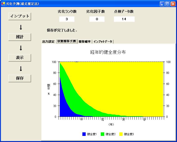
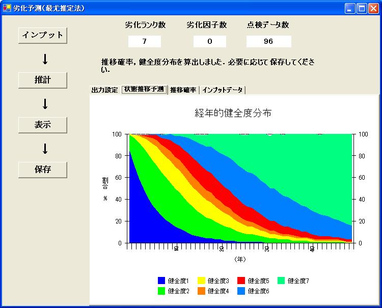
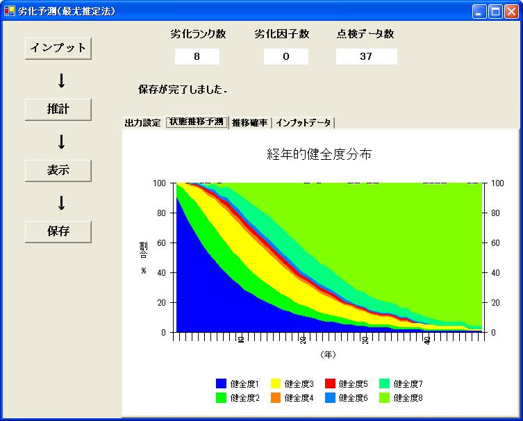
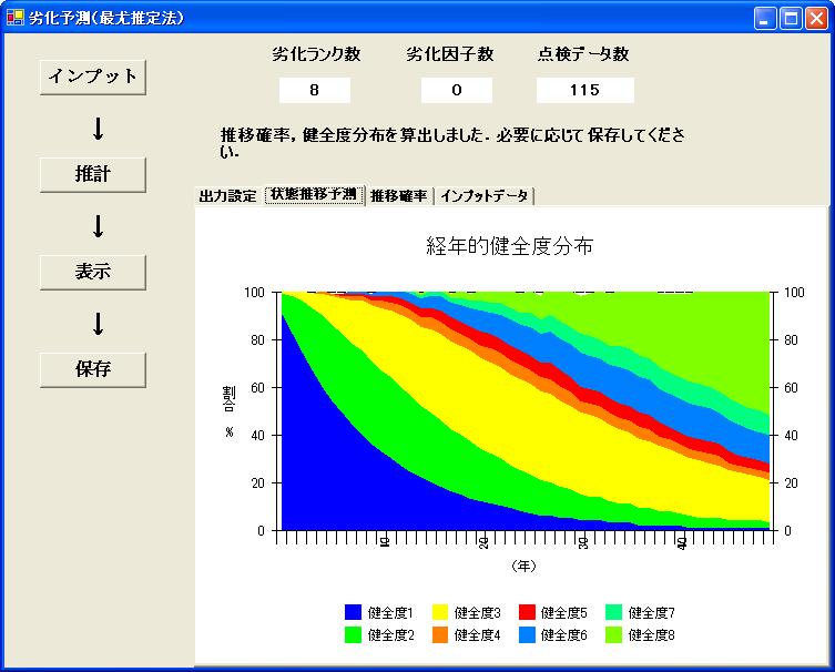
1
2
3 18 1 2,000,000 2,000, (1) 6 JCOSSAR 2007pp
4 LCC (1) (2) 2


5 10mm ,50,60 2 0
6
7
8
9 ) 2) 3) LCC LCC LCC 1
10 1) Vol.42No.5pp ) )
11 LCC 1 3
12
13 6 7 1) 6 JCOSSAR 2007pp
14 1) 3.1 2) RC 3),4) (A) 5)(B) (A)(B) (A) (B),,,, 6
15 3.1 (B) 3.2 6) 7)14) 15) 7
16 X(t+1) t X(t) RC 9) H9 H )14) a,b,c,d,e RC MCI 16)17) 1) pp )
17 3) No pp ) No pp ) ) pp ) JCOSSAR'95 pp , ) RC Vol.47App ) RC 41 4 pp ) RC Vol.7pp ) No pp ) BMS LCC Vol.11pp ) No pp ) No pp ) Hiroshi IIZUKAA STATISTICAL STUDY ON LIFE TIME OF BRIDGESProc. of JSCENo.392-9Vol.5No.1pp.51-60April ) Vol. 63No. 1pp )
18 10
19 11
20 12
21 13
22 A B C D E 14
23 15
24 16
25
26 LCC LCC 18
27 n0,1,2,n=0 n=n N+1 X n 5 Bridge Health Index BHI MCI MCI n n X n
28 5.2.2 RC n=0,1,2, X 0,X 1, 1 2 n-1 X n-1 =i X n-1 X n-1 =i n X n =j p ij p ij n-1 X n-1 =i 20
29 p ij =P(X n =j X n-1 =i),i,js (5.2.1) i j p ij K n-1 n KK i i j
30 n X n =i n=0 n=n' n' X n' =i p in' =P[X n' =i] i K n' K p(n)=p 1n,p 2n,,p Kn n n+1 X n+1 =i n X n i n+1 X n+1 j p ij =P(X n+1 =j X n =i),i,js (5.2.3) 22
31 n+1 X n+1 =j n X n =i p in n X n =i n+1 X n+1 =j p ij p in jn+1 =P(X n =i)p(x n+1 =j X n =i)=p in p ij (5.2.4) p jn+1=p(x n+1 =j)=p in p ij (5.2.5) p 1n+1,p 2n+1,,p Kn+1 = (5.2.6) P(n+1)=p(n)P (5.2.7) n P(n+1)=p(n)P=[p(n-1)P}P ==p(0)[p} n+1 (5.2.8) p(0) P P n X n =i m j p (m) ij p (m) ij i j m p (m) ij (5.2.9) P (m) m m P (m) P m = P (m-1) P= P (m-2) P (2) == PP (m-1) (5.2.10) Chapman-Kolmogorov Chapman-Kolmogorov (5.2.11) 23
32 24
33 25
34 D X Z T = C RC C RC C C C C RC C 1 N ( i = 1, L, N )i J X i = ( X i1, L, X ij) X ij j T = 0 i K S Y i( S) = ( Yi 1( S), L, YiK( S)) Yik ( S) k 26
35 M Z = ( Z 1, L, Z ) Z im m i i im X = ( X 1, L, X ) Z = ( Z 1, L, Z ) i i ij i i im ii ( = 1, K, N) ρ i α ( ) ρ = exp X α + Z β, i = 1, K, N (5.3.1) i i i = ( α1, L, α J ) J = ( 1, L, M ) M β β β N i T T T T (Right Censoring)
36 N T = ( T %, L, 1 T % N) i c i c= ( c1, L, c N ) i T i c i T % i i = 1, L, N if, T% if, T% i i > c i c i (5.3.2) T = 0 c i T = 0 T% i( ci ) Ti = min{ T% i, ci} (5.3.3) i D i D i = 1{ T i = T% i } (5.3.4) i D i 1 if, Ti = T% i( lifetime) = 0 if, Ti = ci( Censoring) (5.3.5) i t λ() t 28
37 Pr( t Ti < t+ t t Ti) λ() t = lim t 0 t (5.3.6) dlog S( t) / dt i T i t St () St () = Pr( t< T i ) (5.3.7) Ft () = 1 St () f () t f () t = ds() t / dt dlog S( t) ds( t) / dt f( t) λ() t = = = (5.3.8) dt S() t S() t f () t = λ() t S() t Λ() t t () t λ( u) du Λ = (5.3.9) 0 St ( ) = exp( Λ ( t)) (5.3.10) v( < t) (Truncation) v Sv () St ()/ Sv ( ), f () t / S( v) f () t / S( v) f() t λ() t = = St ()/ Sv ( ) St () (5.3.11) i T % i f ( T% i) = λ( T% i)exp{ Λ( T% i)} (5.3.12) c i D i = 1Ti = T% i T i f ( T) = λ( T)exp{ Λ ( T)} (5.3.13) i i i D i = 0 T i = c i c i ST ( ) = exp{ Λ ( T)} (5.3.14) i D i = 1 D i = 0 i i = 1, L, N i D l = λ( T) i exp{ Λ( T)} (5.3.15) i i i i 29
38 N N Di L= λ( Ti) exp{ Λ( Ti)} (5.3.16) i= 1 λ() t St () u τ MRL( u) Mean Residual Life MRL( u) = E( τ u u < τ ) (5.3.17) τ u τ τ u u ( t u) f( t) dt u E( τ u u< τ) = (5.3.18) Su ( ) f () t = ds() t / dt [ t ust] ( St ( )) ( t u) f( t) dt = ( t u) [ ds( t) / dt] dt (5.3.19) u u = ( ) ( ) u dt ( t ust ) () ( t ust ) () Stdt () u t t= u u = + (5.3.20) = Stdt () (5.3.21) u t St () u () u MRL( u) = Stdt (5.3.22) Su ( ) t t λ() t t St () 30
39 ρ > 0, t 0 t λ() t ρ t St () exp ( ρt) t λ() t θ θ, ρ > 0,t ρ t t St () ρ θ t θ κ, ρ > 0, t 0 t λ() t ρ exp( κ t) t St () ρ exp 1 exp t κ { ( κ )} 31
40 κ, ρ > 0, t 0 t λ() t κρt 1+ ρt κ 1 κ t St () 1 1+ ρt κ 32
41 κ, ρ > 0, t 0 t λ() t t St () κρ 1 t κ exp ( ρt κ ) T Weibull( ρ, κ) ρ > κ > 0 t 0 λ() t ρκ 1 = t κ (5.3.23) κ > 1 κ = 1 κ < 1 33
42 Λ () t = ρt κ (5.3.24) St ( ) = exp{ Λ ( t)} = exp{ ρt κ } (5.3.25) T κ q q/ κ q ET [ ] = ρ Γ (1 + q/ κ) ET = ρ Γ + / κ (5.3.26) 1/ κ [ ] (1 1 ) Var[ T ] = ρ Γ (1 + 2 / κ) Γ (1 + 1 / κ) (5.3.27) 2/ κ 2 c > 0 T Weibull( ρ, κ ) ct Weibull( ρc κ, κ) T c Weibull( ρ, κ/ c) M Weibull( ρ, κ ) min{ T, L, T M } Weibull( M ρ, κ ) (minimum 1 stable) N 1 D κ i κ L= ρκti ρt i i= 1 exp{ } (5.3.28) N i= 1 log L Dilog( ) Di( 1) logti T κ = ρκ + κ ρ i (5.3.29) κ ρ 34
43 ( 8 t 3.98 ) St ( ) = exp (25%-quantile) (75%-quantile) Su ( ) = exp{ ρu κ } κ exp{ ρt } dt u MRL( u) = (5.3.30) κ exp{ ρu } κ IMRL ( u, ρκ, ) = exp{ ρt } dtκ > 0 y = ρt κ 1 κ dt = t dy/ ( ρκ ) ρ > 0, κ > 0 t y( = ρt κ ) t 1 κ 1 1 / κ 1 / κ 1 u 1 κ (,, ) exp{ } t IMRL u ρκ = y dy (5.3.31) κ ρu ρκ = ρ y 11 / κ (,, ) ρ exp{ } 1/ κ 1 IMRL u ρκ = y y dy κ ρκ (5.3.32) ρu Γ ( ν, z) 1 ( z) exp{ w} w ν ν dw ( ν 0 z 0) z Γ, =, >, > (5.3.33) (,, ) ρ 1 IMRL u ρκ = Γ, u (5.3.34) 1/ κ κ ρ κ κ 35
44 MRL( u) = ρ 1 / 1 κ κ Γ, ρu κ κ κ exp( ρu ) (5.3.35) u = 0 1/ κ ρ 1 0 Γ, / 1 κ κ κ ρ 1 MRL(0) = = Γ, 0 (5.3.36) exp(0) κ κ MRL(0) u 36
45 Y i n Y i µ i µ i > 0 x i k xi = ( xi 1,..., x ik) x i Y i y exp( µ ) i i µ i Pr( Yi = yi µ i) = µ i > 0, yi = 0,1, 2,... (5.4.1) y! i i µ i k µ = exp( x β ) (5.4.2) i β k i 37
46 [ ] =, [ ] E y x µ i i i Var y x = µ (5.4.3) i i i n n y exp( µ ) i i µ i L = (5.4.4) y! i= 1 n µ i y i n n y exp( µ ) i i µ i log L = log i= 1 yi! n i [ µ i yilog( µ i) log( yi!) ] [ exp( x iβ) yix iβ log( yi!) ] (5.4.5) = + = + i= 1 i= 1 n β ˆβ [ ] ˆ E y x = exp( x β ), i = 1,..., n (5.4.6) i i i [ x ] E y i x ij i = ˆ β exp( x ˆ β), i= 1,..., n; j = 1,..., k j i (5.4.7) 38
47 (5.4.6) j x ij 39
48
49 1) , 1998, 20035, 4, 45, 4, 5 4, 4, OK 5, 4, 3, 2, 1 2) 3) i(i=1,,k) S={1,,K} t (t)=i t+1 RC (t+1)=j Pr ob [ ( t + 1) = j( t) = i] = (5.5.1) ij π11 π1k Π = M O M (5.5.2) 0 π KK K j = 1 π = 1 ij RC ς f ς ) F ς ) i i RC i y i+1 λ i ( y i ) y i i ( i i F ~ ( ) i y i i ( i i 41
50 f ( ~ ) i yi yi λ i( yi ) yi = (5.5.3) Fi ( yi) λ i ( y i ) y i i [ y i, y i + y i ] i+1 RC y i θi > 0( i = 1,, K) λ i( yi ) = θi (5.5.4) RC i y F ~ ( ) i i y i ~ F ( y ) = exp( y ) (5.5.5) i i θ i i τ A i y A i y A ~ z ( 0) i F ( y + z ζ y ) ~ F ( y + z ζ y ) i A i i i A i A i i A = Pr ob{ ζ y + z ζ y } (5.5.6) i A i i F ~ ( ) A i y i ~ Fi ( ya + zi) exp{ θ i( ya + zi)} ~ = = exp( θ izi) (5.5.7) Fi ( ya) exp{ θ i ya} y A i y i ω Pr ob[ ( y ) i ( y ) = i] = exp( Z) B ω A θ = (5.5.8) i = y Z B A + Z Pr ob[ ω( y ) = iω( y ) i] B A = π ii π ii θ i Z y A, yb 2) y A y B i j π π = Pr ob[ h( y ) = j h( y ) i] ij B A = ii j m = K = i m= i θ θ θ k 1 j 1 m θm exp( θ kz) θ θ k m= k m+ 1 k (5.5.9) 42
51 K 1 π ik = 1 π ij (5.5.10) j = i π ik
52 5.5.4 H0n =0 n H1n0 t- 1 t t-t t->t n A n305% t )
53 ) 4.62%
54 t
55
56 t- 48
57
58 CLEN
59 CWID
60 HIRW
61 53
62 54
63 55
64 56
65 57
66 58
67 59
68 60
69 61
70 y = 0.020x R² = y = 0.002x R² = 9E mm mm 62
71
72 812mm 0.7mm 1mm 2mm
73 good good 65
74 66
75 67
76 68
77 69
78 70
79 71
80 ,
81 73
82 74
83 75
84 76
85 77
86 78
87 good BIC good good BIC good
88 good BIC good good BIC good
89 good BIC good good BIC good BIC BIC BIC
90 ,50, ,50, ,50,
91 ,50, ,50, ,50,
92 yi y% i =, i= 1,..., n Median( y,..., y ) 1 YDAN 0.12 n
93 YDEP LEVEL µ Dan i Dan µ = exp( β + x β ), i= 1,..., n i L 0 i 1 x L i β 0 β 1 85
94 β 0 β 1 exp( ) = 8.20 µ Pit i µ = exp( β + x β + x β ), i= 1,..., n Pit L Dan i 0 i 1 i 2 x Dan i β 2 x L i β 0 β 1 β 0 β 1 β 2 exp( ) =
95 m -8m -5m -3m -2.5m -1.7m -1m 0m 1.1m 1.8m 1m 1m m -8m -5m -3m -2.5m -1.7m -1m 0m 1.1m 1.8m 6(24mm^2) 20 (80mm^2 ) 87
96 24mm^ mm^2-1m mm^2 88
97 mm^
98 mm^ mm 90
99 50% Tohman-Bain 1 5, 4, 3, 2, t 2.04 t 2.0 (1) c = s r r (1) 91
100 c s r
101
102 94


103 mm 10.2mm 14 40,50, ,50, ,50,60 40,50, ,50, ,50,
104 2 2 1H.C. Shin and S. Madanat : Development of A Stochastic Model of Pavement Distress Initiation, JSCE, No.744/IV-61, pp.61-67, FVol.62, No.2, pp , D.R. Cox and D. Oakes : Analysis of Survival Data, Monographs on Statistics and Applied Probability 21, Chapman & Hall/CRC, E.T. Lee and J.W. Wang : Statistical Methods for Survival Data Analysis, John Wiley & Sons, ) Cox ) :,, W.N. Venables and B.D. Ripley : Modern Applied Statistics with S-PLUS 3rd edition, Chapter12, Springer-Verlag, 1999 ; : S-PLUS,, C. Cameron and P. Trivedi : Econometric Models Based on Count Data : Comparisions and Applications of Some Estimators, Journal of Applied Econometrics, 1, pp.29-53, T. Yasuno : Activity Analysis on Diary Data, K. Kobayashi et al Eds.: Social Capital and Development Trends in Rural Areas, Chap11, :,, ) 2) 96
105 No pp ) Vol.14pp ) 12 pp
106 98 RC
107 RC 99
108 100
109 101
110 102
111 103
112 104
113 105
114 106
115 107
116 108
117 109
118
119
120
121
122 114
123 LCC LCC LCC LCC 1 115
124 (1) (2) 2 116
125 117
Part () () Γ Part ,
 () Γ Part ,") Contents a 6 6 6 6 6 6 6 7 7. 8.. 8.. 8.3. 8 Part. 9. 9.. 9.. 3. 3.. 3.. 3 4. 5 4.. 5 4.. 9 4.3. 3 Part. 6 5. () 6 5.. () 7 5.. 9 5.3. Γ 3 6. 3 6.. 3 6.. 3 6.3. 33 Part 3. 34 7. 34 7.. 34 7.. 34 8. 35
Contents a 6 6 6 6 6 6 6 7 7. 8.. 8.. 8.3. 8 Part. 9. 9.. 9.. 3. 3.. 3.. 3 4. 5 4.. 5 4.. 9 4.3. 3 Part. 6 5. () 6 5.. () 7 5.. 9 5.3. Γ 3 6. 3 6.. 3 6.. 3 6.3. 33 Part 3. 34 7. 34 7.. 34 7.. 34 8. 35
「スウェーデン企業におけるワーク・ライフ・バランス調査 」報告書
 1 2004 12 2005 4 5 100 25 3 1 76 2 Demoskop 2 2004 11 24 30 7 2 10 1 2005 1 31 2 4 5 2 3-1-1 3-1-1 Micromediabanken 2005 1 507 1000 55.0 2 77 50 50 /CEO 36.3 37.4 18.1 3-2-1 43.0 34.4 / 17.6 3-2-2 78 79.4
1 Tokyo Daily Rainfall (mm) Days (mm)
 Days (mm)") ( ) r-taka@maritime.kobe-u.ac.jp 1 Tokyo Daily Rainfall (mm) 0 100 200 300 0 10000 20000 30000 40000 50000 Days (mm) 1876 1 1 2013 12 31 Tokyo, 1876 Daily Rainfall (mm) 0 50 100 150 0 100 200 300 Tokyo,
( ) r-taka@maritime.kobe-u.ac.jp 1 Tokyo Daily Rainfall (mm) 0 100 200 300 0 10000 20000 30000 40000 50000 Days (mm) 1876 1 1 2013 12 31 Tokyo, 1876 Daily Rainfall (mm) 0 50 100 150 0 100 200 300 Tokyo,
2 1,2, , 2 ( ) (1) (2) (3) (4) Cameron and Trivedi(1998) , (1987) (1982) Agresti(2003)
 (1) (2) (3) (4) Cameron and Trivedi(1998) , (1987) (1982) Agresti(2003)") 3 1 1 1 2 1 2 1,2,3 1 0 50 3000, 2 ( ) 1 3 1 0 4 3 (1) (2) (3) (4) 1 1 1 2 3 Cameron and Trivedi(1998) 4 1974, (1987) (1982) Agresti(2003) 3 (1)-(4) AAA, AA+,A (1) (2) (3) (4) (5) (1)-(5) 1 2 5 3 5 (DI)
3 1 1 1 2 1 2 1,2,3 1 0 50 3000, 2 ( ) 1 3 1 0 4 3 (1) (2) (3) (4) 1 1 1 2 3 Cameron and Trivedi(1998) 4 1974, (1987) (1982) Agresti(2003) 3 (1)-(4) AAA, AA+,A (1) (2) (3) (4) (5) (1)-(5) 1 2 5 3 5 (DI)
meiji_resume_1.PDF
 β β β (q 1,q,..., q n ; p 1, p,..., p n ) H(q 1,q,..., q n ; p 1, p,..., p n ) Hψ = εψ ε k = k +1/ ε k = k(k 1) (x, y, z; p x, p y, p z ) (r; p r ), (θ; p θ ), (ϕ; p ϕ ) ε k = 1/ k p i dq i E total = E
TOP URL 1
 TOP URL http://amonphys.web.fc.com/ 3.............................. 3.............................. 4.3 4................... 5.4........................ 6.5........................ 8.6...........................7
201711grade1ouyou.pdf
 2017 11 26 1 2 52 3 12 13 22 23 32 33 42 3 5 3 4 90 5 6 A 1 2 Web Web 3 4 1 2... 5 6 7 7 44 8 9 1 2 3 1 p p >2 2 A 1 2 0.6 0.4 0.52... (a) 0.6 0.4...... B 1 2 0.8-0.2 0.52..... (b) 0.6 0.52.... 1 A B 2
JMP V4 による生存時間分析
 V4 1 SAS 2000.11.18 4 ( ) (Survival Time) 1 (Event) Start of Study Start of Observation Died Died Died Lost End Time Censor Died Died Censor Died Time Start of Study End Start of Observation Censor
医系の統計入門第 2 版 サンプルページ この本の定価 判型などは, 以下の URL からご覧いただけます. このサンプルページの内容は, 第 2 版 1 刷発行時のものです.
 医系の統計入門第 2 版 サンプルページ この本の定価 判型などは, 以下の URL からご覧いただけます. http://www.morikita.co.jp/books/mid/009192 このサンプルページの内容は, 第 2 版 1 刷発行時のものです. i 2 t 1. 2. 3 2 3. 6 4. 7 5. n 2 ν 6. 2 7. 2003 ii 2 2013 10 iii 1987
II ( ) (7/31) II ( [ (3.4)] Navier Stokes [ (6/29)] Navier Stokes 3 [ (6/19)] Re
![II ( ) (7/31) II ( [ (3.4)] Navier Stokes [ (6/29)] Navier Stokes 3 [ (6/19)] Re](/thumbs/94/118770263.jpg "II ( ) (7/31) II ( [ (3.4)] Navier Stokes [ (6/29)] Navier Stokes 3 [ (6/19)] Re") II 29 7 29-7-27 ( ) (7/31) II (http://www.damp.tottori-u.ac.jp/~ooshida/edu/fluid/) [ (3.4)] Navier Stokes [ (6/29)] Navier Stokes 3 [ (6/19)] Reynolds [ (4.6), (45.8)] [ p.186] Navier Stokes I Euler Navier
II 29 7 29-7-27 ( ) (7/31) II (http://www.damp.tottori-u.ac.jp/~ooshida/edu/fluid/) [ (3.4)] Navier Stokes [ (6/29)] Navier Stokes 3 [ (6/19)] Reynolds [ (4.6), (45.8)] [ p.186] Navier Stokes I Euler Navier
 2011 8 26 3 I 5 1 7 1.1 Markov................................ 7 2 Gau 13 2.1.................................. 13 2.2............................... 18 2.3............................ 23 3 Gau (Le vy
Z: Q: R: C: sin 6 5 ζ a, b
 Z: Q: R: C: 3 3 7 4 sin 6 5 ζ 9 6 6............................... 6............................... 6.3......................... 4 7 6 8 8 9 3 33 a, b a bc c b a a b 5 3 5 3 5 5 3 a a a a p > p p p, 3,

2 1 1 α = a + bi(a, b R) α (conjugate) α = a bi α (absolute value) α = a 2 + b 2 α (norm) N(α) = a 2 + b 2 = αα = α 2 α (spure) (trace) 1 1. a R aα =
 α (conjugate) α = a bi α (absolute value) α = a 2 + b 2 α (norm) N(α) = a 2 + b 2 = αα = α 2 α (spure) (trace) 1 1. a R aα =") 1 1 α = a + bi(a, b R) α (conjugate) α = a bi α (absolute value) α = a + b α (norm) N(α) = a + b = αα = α α (spure) (trace) 1 1. a R aα = aα. α = α 3. α + β = α + β 4. αβ = αβ 5. β 0 6. α = α ( ) α = α
1 1 α = a + bi(a, b R) α (conjugate) α = a bi α (absolute value) α = a + b α (norm) N(α) = a + b = αα = α α (spure) (trace) 1 1. a R aα = aα. α = α 3. α + β = α + β 4. αβ = αβ 5. β 0 6. α = α ( ) α = α
I A A441 : April 15, 2013 Version : 1.1 I Kawahira, Tomoki TA (Shigehiro, Yoshida )
") I013 00-1 : April 15, 013 Version : 1.1 I Kawahira, Tomoki TA (Shigehiro, Yoshida) http://www.math.nagoya-u.ac.jp/~kawahira/courses/13s-tenbou.html pdf * 4 15 4 5 13 e πi = 1 5 0 5 7 3 4 6 3 6 10 6 17
I013 00-1 : April 15, 013 Version : 1.1 I Kawahira, Tomoki TA (Shigehiro, Yoshida) http://www.math.nagoya-u.ac.jp/~kawahira/courses/13s-tenbou.html pdf * 4 15 4 5 13 e πi = 1 5 0 5 7 3 4 6 3 6 10 6 17
) a + b = i + 6 b c = 6i j ) a = 0 b = c = 0 ) â = i + j 0 ˆb = 4) a b = b c = j + ) cos α = cos β = 6) a ˆb = b ĉ = 0 7) a b = 6i j b c = i + 6j + 8)
 a + b = i + 6 b c = 6i j ) a = 0 b = c = 0 ) â = i + j 0 ˆb = 4) a b = b c = j + ) cos α = cos β = 6) a ˆb = b ĉ = 0 7) a b = 6i j b c = i + 6j + 8)") 4 4 ) a + b = i + 6 b c = 6i j ) a = 0 b = c = 0 ) â = i + j 0 ˆb = 4) a b = b c = j + ) cos α = cos β = 6) a ˆb = b ĉ = 0 7) a b = 6i j b c = i + 6j + 8) a b a b = 6i j 4 b c b c 9) a b = 4 a b) c = 7
4 4 ) a + b = i + 6 b c = 6i j ) a = 0 b = c = 0 ) â = i + j 0 ˆb = 4) a b = b c = j + ) cos α = cos β = 6) a ˆb = b ĉ = 0 7) a b = 6i j b c = i + 6j + 8) a b a b = 6i j 4 b c b c 9) a b = 4 a b) c = 7
,,,17,,, ( ),, E Q [S T F t ] < S t, t [, T ],,,,,,,,
![,,,17,,, ( ),, E Q [S T F t ] < S t, t [, T ],,,,,,,,](/thumbs/91/105754403.jpg ",,,17,,, ( ),, E Q [S T F t ] < S t, t [, T ],,,,,,,,") 14 5 1 ,,,17,,,194 1 4 ( ),, E Q [S T F t ] < S t, t [, T ],,,,,,,, 1 4 1.1........................................ 4 5.1........................................ 5.........................................
14 5 1 ,,,17,,,194 1 4 ( ),, E Q [S T F t ] < S t, t [, T ],,,,,,,, 1 4 1.1........................................ 4 5.1........................................ 5.........................................
chap9.dvi
 9 AR (i) (ii) MA (iii) (iv) (v) 9.1 2 1 AR 1 9.1.1 S S y j = (α i + β i j) D ij + η j, η j = ρ S η j S + ε j (j =1,,T) (1) i=1 {ε j } i.i.d(,σ 2 ) η j (j ) D ij j i S 1 S =1 D ij =1 S>1 S =4 (1) y j =
 http://www.ike-dyn.ritsumei.ac.jp/ hyoo/wave.html 1 1, 5 3 1.1 1..................................... 3 1.2 5.1................................... 4 1.3.......................... 5 1.4 5.2, 5.3....................

ii 3.,. 4. F. (), ,,. 8.,. 1. (75%) (25%) =7 20, =7 21 (. ). 1.,, (). 3.,. 1. ().,.,.,.,.,. () (12 )., (), 0. 2., 1., 0,.
, ,,. 8.,. 1. (75%) (25%) =7 20, =7 21 (. ). 1.,, (). 3.,. 1. ().,.,.,.,.,. () (12 )., (), 0. 2., 1., 0,.") 24(2012) (1 C106) 4 11 (2 C206) 4 12 http://www.math.is.tohoku.ac.jp/~obata,.,,,.. 1. 2. 3. 4. 5. 6. 7.,,. 1., 2007 (). 2. P. G. Hoel, 1995. 3... 1... 2.,,. ii 3.,. 4. F. (),.. 5... 6.. 7.,,. 8.,. 1. (75%)
24(2012) (1 C106) 4 11 (2 C206) 4 12 http://www.math.is.tohoku.ac.jp/~obata,.,,,.. 1. 2. 3. 4. 5. 6. 7.,,. 1., 2007 (). 2. P. G. Hoel, 1995. 3... 1... 2.,,. ii 3.,. 4. F. (),.. 5... 6.. 7.,,. 8.,. 1. (75%)
2 G(k) e ikx = (ik) n x n n! n=0 (k ) ( ) X n = ( i) n n k n G(k) k=0 F (k) ln G(k) = ln e ikx n κ n F (k) = F (k) (ik) n n= n! κ n κ n = ( i) n n k n
 e ikx = (ik) n x n n! n=0 (k ) ( ) X n = ( i) n n k n G(k) k=0 F (k) ln G(k) = ln e ikx n κ n F (k) = F (k) (ik) n n= n! κ n κ n = ( i) n n k n") . X {x, x 2, x 3,... x n } X X {, 2, 3, 4, 5, 6} X x i P i. 0 P i 2. n P i = 3. P (i ω) = i ω P i P 3 {x, x 2, x 3,... x n } ω P i = 6 X f(x) f(x) X n n f(x i )P i n x n i P i X n 2 G(k) e ikx = (ik) n
. X {x, x 2, x 3,... x n } X X {, 2, 3, 4, 5, 6} X x i P i. 0 P i 2. n P i = 3. P (i ω) = i ω P i P 3 {x, x 2, x 3,... x n } ω P i = 6 X f(x) f(x) X n n f(x i )P i n x n i P i X n 2 G(k) e ikx = (ik) n
simx simxdx, cosxdx, sixdx 6.3 px m m + pxfxdx = pxf x p xf xdx = pxf x p xf x + p xf xdx 7.4 a m.5 fx simxdx 8 fx fx simxdx = πb m 9 a fxdx = πa a =
 II 6 ishimori@phys.titech.ac.jp 6.. 5.4.. f Rx = f Lx = fx fx + lim = lim x x + x x f c = f x + x < c < x x x + lim x x fx fx x x = lim x x f c = f x x < c < x cosmx cosxdx = {cosm x + cosm + x} dx = [
4. ϵ(ν, T ) = c 4 u(ν, T ) ϵ(ν, T ) T ν π4 Planck dx = 0 e x 1 15 U(T ) x 3 U(T ) = σt 4 Stefan-Boltzmann σ 2π5 k 4 15c 2 h 3 = W m 2 K 4 5.
 = c 4 u(ν, T ) ϵ(ν, T ) T ν π4 Planck dx = 0 e x 1 15 U(T ) x 3 U(T ) = σt 4 Stefan-Boltzmann σ 2π5 k 4 15c 2 h 3 = W m 2 K 4 5.") A 1. Boltzmann Planck u(ν, T )dν = 8πh ν 3 c 3 kt 1 dν h 6.63 10 34 J s Planck k 1.38 10 23 J K 1 Boltzmann u(ν, T ) T ν e hν c = 3 10 8 m s 1 2. Planck λ = c/ν Rayleigh-Jeans u(ν, T )dν = 8πν2 kt dν c
A 1. Boltzmann Planck u(ν, T )dν = 8πh ν 3 c 3 kt 1 dν h 6.63 10 34 J s Planck k 1.38 10 23 J K 1 Boltzmann u(ν, T ) T ν e hν c = 3 10 8 m s 1 2. Planck λ = c/ν Rayleigh-Jeans u(ν, T )dν = 8πν2 kt dν c
( ) 2.1. C. (1) x 4 dx = 1 5 x5 + C 1 (2) x dx = x 2 dx = x 1 + C = 1 2 x + C xdx (3) = x dx = 3 x C (4) (x + 1) 3 dx = (x 3 + 3x 2 + 3x +
 2.1. C. (1) x 4 dx = 1 5 x5 + C 1 (2) x dx = x 2 dx = x 1 + C = 1 2 x + C xdx (3) = x dx = 3 x C (4) (x + 1) 3 dx = (x 3 + 3x 2 + 3x +") (.. C. ( d 5 5 + C ( d d + C + C d ( d + C ( ( + d ( + + + d + + + + C (5 9 + d + d tan + C cos (sin (6 sin d d log sin + C sin + (7 + + d ( + + + + d log( + + + C ( (8 d 7 6 d + 6 + C ( (9 ( d 6 + 8 d
(.. C. ( d 5 5 + C ( d d + C + C d ( d + C ( ( + d ( + + + d + + + + C (5 9 + d + d tan + C cos (sin (6 sin d d log sin + C sin + (7 + + d ( + + + + d log( + + + C ( (8 d 7 6 d + 6 + C ( (9 ( d 6 + 8 d
9 5 ( α+ ) = (α + ) α (log ) = α d = α C d = log + C C 5. () d = 4 d = C = C = 3 + C 3 () d = d = C = C = 3 + C 3 =
 = (α + ) α (log ) = α d = α C d = log + C C 5. () d = 4 d = C = C = 3 + C 3 () d = d = C = C = 3 + C 3 =") 5 5. 5.. A II f() f() F () f() F () = f() C (F () + C) = F () = f() F () + C f() F () G() f() G () = F () 39 G() = F () + C C f() F () f() F () + C C f() f() d f() f() C f() f() F () = f() f() f() d =
5 5. 5.. A II f() f() F () f() F () = f() C (F () + C) = F () = f() F () + C f() F () G() f() G () = F () 39 G() = F () + C C f() F () f() F () + C C f() f() d f() f() C f() f() F () = f() f() f() d =
( ) Loewner SLE 13 February
 Loewner SLE 13 February") ( ) Loewner SLE 3 February 00 G. F. Lawler, Conformally Invariant Processes in the Plane, (American Mathematical Society, 005)., Summer School 009 (009 8 7-9 ) . d- (BES d ) d B t = (Bt, B t,, Bd t ) (d
( ) Loewner SLE 3 February 00 G. F. Lawler, Conformally Invariant Processes in the Plane, (American Mathematical Society, 005)., Summer School 009 (009 8 7-9 ) . d- (BES d ) d B t = (Bt, B t,, Bd t ) (d
5 Armitage x 1,, x n y i = 10x i + 3 y i = log x i {x i } {y i } 1.2 n i i x ij i j y ij, z ij i j 2 1 y = a x + b ( cm) x ij (i j )
 x ij (i j )") 5 Armitage. x,, x n y i = 0x i + 3 y i = log x i x i y i.2 n i i x ij i j y ij, z ij i j 2 y = a x + b 2 2. ( cm) x ij (i j ) (i) x, x 2 σ 2 x,, σ 2 x,2 σ x,, σ x,2 t t x * (ii) (i) m y ij = x ij /00 y
5 Armitage. x,, x n y i = 0x i + 3 y i = log x i x i y i.2 n i i x ij i j y ij, z ij i j 2 y = a x + b 2 2. ( cm) x ij (i j ) (i) x, x 2 σ 2 x,, σ 2 x,2 σ x,, σ x,2 t t x * (ii) (i) m y ij = x ij /00 y
変 位 変位とは 物体中のある点が変形後に 別の点に異動したときの位置の変化で あり ベクトル量である 変位には 物体の変形の他に剛体運動 剛体変位 が含まれている 剛体変位 P(x, y, z) 平行移動と回転 P! (x + u, y + v, z + w) Q(x + d x, y + dy,
 平行移動と回転 P! (x + u, y + v, z + w) Q(x + d x, y + dy,") 変 位 変位とは 物体中のある点が変形後に 別の点に異動したときの位置の変化で あり ベクトル量である 変位には 物体の変形の他に剛体運動 剛体変位 が含まれている 剛体変位 P(x, y, z) 平行移動と回転 P! (x + u, y + v, z + w) Q(x + d x, y + dy, z + dz) Q! (x + d x + u + du, y + dy + v + dv, z +
変 位 変位とは 物体中のある点が変形後に 別の点に異動したときの位置の変化で あり ベクトル量である 変位には 物体の変形の他に剛体運動 剛体変位 が含まれている 剛体変位 P(x, y, z) 平行移動と回転 P! (x + u, y + v, z + w) Q(x + d x, y + dy, z + dz) Q! (x + d x + u + du, y + dy + v + dv, z +
 n ξ n,i, i = 1,, n S n ξ n,i n 0 R 1,.. σ 1 σ i .10.14.15 0 1 0 1 1 3.14 3.18 3.19 3.14 3.14,. ii 1 1 1.1..................................... 1 1............................... 3 1.3.........................
chap10.dvi
 . q {y j } I( ( L y j =Δy j = u j = C l ε j l = C(L ε j, {ε j } i.i.d.(,i q ( l= y O p ( {u j } q {C l } A l C l
untitled
 2 : n =1, 2,, 10000 0.5125 0.51 0.5075 0.505 0.5025 0.5 0.4975 0.495 0 2000 4000 6000 8000 10000 2 weak law of large numbers 1. X 1,X 2,,X n 2. µ = E(X i ),i=1, 2,,n 3. σi 2 = V (X i ) σ 2,i=1, 2,,n ɛ>0
S I. dy fx x fx y fx + C 3 C dy fx 4 x, y dy v C xt y C v e kt k > xt yt gt [ v dt dt v e kt xt v e kt + C k x v + C C k xt v k 3 r r + dr e kt S dt d
 S I.. http://ayapin.film.s.dendai.ac.jp/~matuda /TeX/lecture.html PDF PS.................................... 3.3.................... 9.4................5.............. 3 5. Laplace................. 5....
: , 2.0, 3.0, 2.0, (%) ( 2.
 ( 2.") 2017 1 2 1.1...................................... 2 1.2......................................... 4 1.3........................................... 10 1.4................................. 14 1.5..........................................
2017 1 2 1.1...................................... 2 1.2......................................... 4 1.3........................................... 10 1.4................................. 14 1.5..........................................
(2) Fisher α (α) α Fisher α ( α) 0 Levi Civita (1) ( 1) e m (e) (m) ([1], [2], [13]) Poincaré e m Poincaré e m Kähler-like 2 Kähler-like
![(2) Fisher α (α) α Fisher α ( α) 0 Levi Civita (1) ( 1) e m (e) (m) ([1], [2], [13]) Poincaré e m Poincaré e m Kähler-like 2 Kähler-like](/thumbs/97/133596579.jpg "(2) Fisher α (α) α Fisher α ( α) 0 Levi Civita (1) ( 1) e m (e) (m) ([1], [2], [13]) Poincaré e m Poincaré e m Kähler-like 2 Kähler-like") () 10 9 30 1 Fisher α (α) α Fisher α ( α) 0 Levi Civita (1) ( 1) e m (e) (m) ([1], [], [13]) Poincaré e m Poincaré e m Kähler-like Kähler-like Kähler M g M X, Y, Z (.1) Xg(Y, Z) = g( X Y, Z) + g(y, XZ)
() 10 9 30 1 Fisher α (α) α Fisher α ( α) 0 Levi Civita (1) ( 1) e m (e) (m) ([1], [], [13]) Poincaré e m Poincaré e m Kähler-like Kähler-like Kähler M g M X, Y, Z (.1) Xg(Y, Z) = g( X Y, Z) + g(y, XZ)
‚åŁÎ“·„´Šš‡ðŠp‡¢‡½‹âfi`fiI…A…‰…S…−…Y…•‡ÌMarkovŸA“½fiI›ð’Í
 Markov 2009 10 2 Markov 2009 10 2 1 / 25 1 (GA) 2 GA 3 4 Markov 2009 10 2 2 / 25 (GA) (GA) L ( 1) I := {0, 1} L f : I (0, ) M( 2) S := I M GA (GA) f (i) i I Markov 2009 10 2 3 / 25 (GA) ρ(i, j), i, j I
構造と連続体の力学基礎
 II 37 Wabash Avenue Bridge, Illinois 州 Winnipeg にある歩道橋 Esplanade Riel 橋6 6 斜張橋である必要は多分無いと思われる すぐ横に道路用桁橋有り しかも塔基部のレストランは 8 年には営業していなかった 9 9. 9.. () 97 [3] [5] k 9. m w(t) f (t) = f (t) + mg k w(t) Newton
 1 1 1 1-1 1 1-9 1-3 1-1 13-17 -3 6-4 6 3 3-1 35 3-37 3-3 38 4 4-1 39 4- Fe C TEM 41 4-3 C TEM 44 4-4 Fe TEM 46 4-5 5 4-6 5 5 51 6 5 1 1-1 1991 1,1 multiwall nanotube 1993 singlewall nanotube ( 1,) sp 7.4eV
(1.2) T D = 0 T = D = 30 kn 1.2 (1.4) 2F W = 0 F = W/2 = 300 kn/2 = 150 kn 1.3 (1.9) R = W 1 + W 2 = = 1100 N. (1.9) W 2 b W 1 a = 0
 T D = 0 T = D = 30 kn 1.2 (1.4) 2F W = 0 F = W/2 = 300 kn/2 = 150 kn 1.3 (1.9) R = W 1 + W 2 = = 1100 N. (1.9) W 2 b W 1 a = 0") 1 1 1.1 1.) T D = T = D = kn 1. 1.4) F W = F = W/ = kn/ = 15 kn 1. 1.9) R = W 1 + W = 6 + 5 = 11 N. 1.9) W b W 1 a = a = W /W 1 )b = 5/6) = 5 cm 1.4 AB AC P 1, P x, y x, y y x 1.4.) P sin 6 + P 1 sin 45
1 1 1.1 1.) T D = T = D = kn 1. 1.4) F W = F = W/ = kn/ = 15 kn 1. 1.9) R = W 1 + W = 6 + 5 = 11 N. 1.9) W b W 1 a = a = W /W 1 )b = 5/6) = 5 cm 1.4 AB AC P 1, P x, y x, y y x 1.4.) P sin 6 + P 1 sin 45
gr09.dvi
 .1, θ, ϕ d = A, t dt + B, t dtd + C, t d + D, t dθ +in θdϕ.1.1 t { = f1,t t = f,t { D, t = B, t =.1. t A, tdt e φ,t dt, C, td e λ,t d.1.3,t, t d = e φ,t dt + e λ,t d + dθ +in θdϕ.1.4 { = f1,t t = f,t {
..3. Ω, Ω F, P Ω, F, P ). ) F a) A, A,..., A i,... F A i F. b) A F A c F c) Ω F. ) A F A P A),. a) 0 P A) b) P Ω) c) [ ] A, A,..., A i,... F i j A i A
![..3. Ω, Ω F, P Ω, F, P ). ) F a) A, A,..., A i,... F A i F. b) A F A c F c) Ω F. ) A F A P A),. a) 0 P A) b) P Ω) c) [ ] A, A,..., A i,... F i j A i A](/thumbs/93/112175219.jpg "..3. Ω, Ω F, P Ω, F, P ). ) F a) A, A,..., A i,... F A i F. b) A F A c F c) Ω F. ) A F A P A),. a) 0 P A) b) P Ω) c) [ ] A, A,..., A i,... F i j A i A") .. Laplace ). A... i),. ω i i ). {ω,..., ω } Ω,. ii) Ω. Ω. A ) r, A P A) P A) r... ).. Ω {,, 3, 4, 5, 6}. i i 6). A {, 4, 6} P A) P A) 3 6. ).. i, j i, j) ) Ω {i, j) i 6, j 6}., 36. A. A {i, j) i j }.
.. Laplace ). A... i),. ω i i ). {ω,..., ω } Ω,. ii) Ω. Ω. A ) r, A P A) P A) r... ).. Ω {,, 3, 4, 5, 6}. i i 6). A {, 4, 6} P A) P A) 3 6. ).. i, j i, j) ) Ω {i, j) i 6, j 6}., 36. A. A {i, j) i j }.
waseda2010a-jukaiki1-main.dvi
 November, 2 Contents 6 2 8 3 3 3 32 32 33 5 34 34 6 35 35 7 4 R 2 7 4 4 9 42 42 2 43 44 2 5 : 2 5 5 23 52 52 23 53 53 23 54 24 6 24 6 6 26 62 62 26 63 t 27 7 27 7 7 28 72 72 28 73 36) 29 8 29 8 29 82 3
ii 3.,. 4. F. ( ), ,,. 8.,. 1. (75% ) (25% ) =7 24, =7 25, =7 26 (. ). 1.,, ( ). 3.,...,.,.,.,.,. ( ) (1 2 )., ( ), 0., 1., 0,.
, ,,. 8.,. 1. (75% ) (25% ) =7 24, =7 25, =7 26 (. ). 1.,, ( ). 3.,...,.,.,.,.,. ( ) (1 2 )., ( ), 0., 1., 0,.") (1 C205) 4 10 (2 C206) 4 11 (2 B202) 4 12 25(2013) http://www.math.is.tohoku.ac.jp/~obata,.,,,..,,. 1. 2. 3. 4. 5. 6. 7. 8. 1., 2007 ( ).,. 2. P. G., 1995. 3. J. C., 1988. 1... 2.,,. ii 3.,. 4. F. ( ),..
(1 C205) 4 10 (2 C206) 4 11 (2 B202) 4 12 25(2013) http://www.math.is.tohoku.ac.jp/~obata,.,,,..,,. 1. 2. 3. 4. 5. 6. 7. 8. 1., 2007 ( ).,. 2. P. G., 1995. 3. J. C., 1988. 1... 2.,,. ii 3.,. 4. F. ( ),..
,. Black-Scholes u t t, x c u 0 t, x x u t t, x c u t, x x u t t, x + σ x u t, x + rx ut, x rux, t 0 x x,,.,. Step 3, 7,,, Step 6., Step 4,. Step 5,,.
 9 α ν β Ξ ξ Γ γ o δ Π π ε ρ ζ Σ σ η τ Θ θ Υ υ ι Φ φ κ χ Λ λ Ψ ψ µ Ω ω Def, Prop, Th, Lem, Note, Remark, Ex,, Proof, R, N, Q, C [a, b {x R : a x b} : a, b {x R : a < x < b} : [a, b {x R : a x < b} : a,
.2 ρ dv dt = ρk grad p + 3 η grad (divv) + η 2 v.3 divh = 0, rote + c H t = 0 dive = ρ, H = 0, E = ρ, roth c E t = c ρv E + H c t = 0 H c E t = c ρv T
 + η 2 v.3 divh = 0, rote + c H t = 0 dive = ρ, H = 0, E = ρ, roth c E t = c ρv E + H c t = 0 H c E t = c ρv T") NHK 204 2 0 203 2 24 ( ) 7 00 7 50 203 2 25 ( ) 7 00 7 50 203 2 26 ( ) 7 00 7 50 203 2 27 ( ) 7 00 7 50 I. ( ν R n 2 ) m 2 n m, R = e 2 8πε 0 hca B =.09737 0 7 m ( ν = ) λ a B = 4πε 0ħ 2 m e e 2 = 5.2977
NHK 204 2 0 203 2 24 ( ) 7 00 7 50 203 2 25 ( ) 7 00 7 50 203 2 26 ( ) 7 00 7 50 203 2 27 ( ) 7 00 7 50 I. ( ν R n 2 ) m 2 n m, R = e 2 8πε 0 hca B =.09737 0 7 m ( ν = ) λ a B = 4πε 0ħ 2 m e e 2 = 5.2977
keisoku01.dvi
 2.,, Mon, 2006, 401, SAGA, JAPAN Dept. of Mechanical Engineering, Saga Univ., JAPAN 4 Mon, 2006, 401, SAGA, JAPAN Dept. of Mechanical Engineering, Saga Univ., JAPAN 5 Mon, 2006, 401, SAGA, JAPAN Dept.
Hanbury-Brown Twiss (ver. 2.0) van Cittert - Zernike mutual coherence
 van Cittert - Zernike mutual coherence") Hanbury-Brown Twiss (ver. 2.) 25 4 4 1 2 2 2 2.1 van Cittert - Zernike..................................... 2 2.2 mutual coherence................................. 4 3 Hanbury-Brown Twiss ( ) 5 3.1............................................
Hanbury-Brown Twiss (ver. 2.) 25 4 4 1 2 2 2 2.1 van Cittert - Zernike..................................... 2 2.2 mutual coherence................................. 4 3 Hanbury-Brown Twiss ( ) 5 3.1............................................
微分積分 サンプルページ この本の定価 判型などは, 以下の URL からご覧いただけます. このサンプルページの内容は, 初版 1 刷発行時のものです.
 微分積分 サンプルページ この本の定価 判型などは, 以下の URL からご覧いただけます. ttp://www.morikita.co.jp/books/mid/00571 このサンプルページの内容は, 初版 1 刷発行時のものです. i ii 014 10 iii [note] 1 3 iv 4 5 3 6 4 x 0 sin x x 1 5 6 z = f(x, y) 1 y = f(x)
(2004 ) 2 (A) (B) (C) 3 (1987) (1988) Shimono and Tachibanaki(1985) (2008) , % 2 (1999) (2005) 3 (2005) (2006) (2008)
 2 (A) (B) (C) 3 (1987) (1988) Shimono and Tachibanaki(1985) (2008) , % 2 (1999) (2005) 3 (2005) (2006) (2008)") ,, 23 4 30 (i) (ii) (i) (ii) Negishi (1960) 2010 (2010) ( ) ( ) (2010) E-mail:fujii@econ.kobe-u.ac.jp E-mail:082e527e@stu.kobe-u.ac.jp E-mail:iritani@econ.kobe-u.ac.jp 1 1 16 (2004 ) 2 (A) (B) (C) 3 (1987)
,, 23 4 30 (i) (ii) (i) (ii) Negishi (1960) 2010 (2010) ( ) ( ) (2010) E-mail:fujii@econ.kobe-u.ac.jp E-mail:082e527e@stu.kobe-u.ac.jp E-mail:iritani@econ.kobe-u.ac.jp 1 1 16 (2004 ) 2 (A) (B) (C) 3 (1987)
ohpmain.dvi
 fujisawa@ism.ac.jp 1 Contents 1. 2. 3. 4. γ- 2 1. 3 10 5.6, 5.7, 5.4, 5.5, 5.8, 5.5, 5.3, 5.6, 5.4, 5.2. 5.5 5.6 +5.7 +5.4 +5.5 +5.8 +5.5 +5.3 +5.6 +5.4 +5.2 =5.5. 10 outlier 5 5.6, 5.7, 5.4, 5.5, 5.8,
seminar0220a.dvi
 1 Hi-Stat 2 16 2 20 16:30-18:00 2 2 217 1 COE 4 COE RA E-MAIL: ged0104@srv.cc.hit-u.ac.jp 2004 2 25 S-PLUS S-PLUS S-PLUS S-code 2 [8] [8] [8] 1 2 ARFIMA(p, d, q) FI(d) φ(l)(1 L) d x t = θ(l)ε t ({ε t }
S I. dy fx x fx y fx + C 3 C vt dy fx 4 x, y dy yt gt + Ct + C dt v e kt xt v e kt + C k x v k + C C xt v k 3 r r + dr e kt S Sr πr dt d v } dt k e kt
 S I. x yx y y, y,. F x, y, y, y,, y n http://ayapin.film.s.dendai.ac.jp/~matuda n /TeX/lecture.html PDF PS yx.................................... 3.3.................... 9.4................5..............
Untitled
 II 14 14-7-8 8/4 II (http://www.damp.tottori-u.ac.jp/~ooshida/edu/fluid/) [ (3.4)] Navier Stokes [ 6/ ] Navier Stokes 3 [ ] Reynolds [ (4.6), (45.8)] [ p.186] Navier Stokes I 1 balance law t (ρv i )+ j
Venkatram and Wyngaard, Lectures on Air Pollution Modeling, m km 6.2 Stull, An Introduction to Boundary Layer Meteorology,
 65 6 6.1 No.4 1982 1 1981 J. C. Kaimal 1993 1994 Turbulence and Diffusion in the Atmosphere : Lectures in Environmental Sciences, by A. K. Blackadar, Springer, 1998 An Introduction to Boundary Layer Meteorology,
() n C + n C + n C + + n C n n (3) n C + n C + n C 4 + n C + n C 3 + n C 5 + (5) (6 ) n C + nc + 3 nc n nc n (7 ) n C + nc + 3 nc n nc n (
 n C + n C + n C + + n C n n (3) n C + n C + n C 4 + n C + n C 3 + n C 5 + (5) (6 ) n C + nc + 3 nc n nc n (7 ) n C + nc + 3 nc n nc n (") 3 n nc k+ k + 3 () n C r n C n r nc r C r + C r ( r n ) () n C + n C + n C + + n C n n (3) n C + n C + n C 4 + n C + n C 3 + n C 5 + (4) n C n n C + n C + n C + + n C n (5) k k n C k n C k (6) n C + nc
3 n nc k+ k + 3 () n C r n C n r nc r C r + C r ( r n ) () n C + n C + n C + + n C n n (3) n C + n C + n C 4 + n C + n C 3 + n C 5 + (4) n C n n C + n C + n C + + n C n (5) k k n C k n C k (6) n C + nc
10:30 12:00 P.G. vs vs vs 2
 1 10:30 12:00 P.G. vs vs vs 2 LOGIT PROBIT TOBIT mean median mode CV 3 4 5 0.5 1000 6 45 7 P(A B) = P(A) + P(B) - P(A B) P(B A)=P(A B)/P(A) P(A B)=P(B A) P(A) P(A B) P(A) P(B A) P(B) P(A B) P(A) P(B) P(B
量子力学 問題
 3 : 203 : 0. H = 0 0 2 6 0 () = 6, 2 = 2, 3 = 3 3 H 6 2 3 ϵ,2,3 (2) ψ = (, 2, 3 ) ψ Hψ H (3) P i = i i P P 2 = P 2 P 3 = P 3 P = O, P 2 i = P i (4) P + P 2 + P 3 = E 3 (5) i ϵ ip i H 0 0 (6) R = 0 0 [H,
II No.01 [n/2] [1]H n (x) H n (x) = ( 1) r n! r!(n 2r)! (2x)n 2r. r=0 [2]H n (x) n,, H n ( x) = ( 1) n H n (x). [3] H n (x) = ( 1) n dn x2 e dx n e x2
![II No.01 [n/2] [1]H n (x) H n (x) = ( 1) r n! r!(n 2r)! (2x)n 2r. r=0 [2]H n (x) n,, H n ( x) = ( 1) n H n (x). [3] H n (x) = ( 1) n dn x2 e dx n e x2](/thumbs/101/149159646.jpg "II No.01 [n/2] [1]H n (x) H n (x) = ( 1) r n! r!(n 2r)! (2x)n 2r. r=0 [2]H n (x) n,, H n ( x) = ( 1) n H n (x). [3] H n (x) = ( 1) n dn x2 e dx n e x2") II No.1 [n/] [1]H n x) H n x) = 1) r n! r!n r)! x)n r r= []H n x) n,, H n x) = 1) n H n x) [3] H n x) = 1) n dn x e dx n e x [4] H n+1 x) = xh n x) nh n 1 x) ) d dx x H n x) = H n+1 x) d dx H nx) = nh
II No.1 [n/] [1]H n x) H n x) = 1) r n! r!n r)! x)n r r= []H n x) n,, H n x) = 1) n H n x) [3] H n x) = 1) n dn x e dx n e x [4] H n+1 x) = xh n x) nh n 1 x) ) d dx x H n x) = H n+1 x) d dx H nx) = nh
6.1 (P (P (P (P (P (P (, P (, P.
 (011 30 7 0 ( ( 3 ( 010 1 (P.3 1 1.1 (P.4.................. 1 1. (P.4............... 1 (P.15.1 (P.16................. (P.0............3 (P.18 3.4 (P.3............... 4 3 (P.9 4 3.1 (P.30........... 4 3.
( ) ,
 ,") II 2007 4 0. 0 1 0 2 ( ) 0 3 1 2 3 4, - 5 6 7 1 1 1 1 1) 2) 3) 4) ( ) () H 2.79 10 10 He 2.72 10 9 C 1.01 10 7 N 3.13 10 6 O 2.38 10 7 Ne 3.44 10 6 Mg 1.076 10 6 Si 1 10 6 S 5.15 10 5 Ar 1.01 10 5 Fe 9.00
II 2007 4 0. 0 1 0 2 ( ) 0 3 1 2 3 4, - 5 6 7 1 1 1 1 1) 2) 3) 4) ( ) () H 2.79 10 10 He 2.72 10 9 C 1.01 10 7 N 3.13 10 6 O 2.38 10 7 Ne 3.44 10 6 Mg 1.076 10 6 Si 1 10 6 S 5.15 10 5 Ar 1.01 10 5 Fe 9.00
Kullback-Leibler
 Kullback-Leibler 206 6 6 http://www.math.tohoku.ac.jp/~kuroki/latex/206066kullbackleibler.pdf 0 2 Kullback-Leibler 3. q i.......................... 3.2........... 3.3 Kullback-Leibler.............. 4.4
: : : : ) ) 1. d ij f i e i x i v j m a ij m f ij n x i =
 ) 1. d ij f i e i x i v j m a ij m f ij n x i =") 1 1980 1) 1 2 3 19721960 1965 2) 1999 1 69 1980 1972: 55 1999: 179 2041999: 210 211 1999: 211 3 2003 1987 92 97 3) 1960 1965 1970 1985 1990 1995 4) 1. d ij f i e i x i v j m a ij m f ij n x i = n d ij
1 1980 1) 1 2 3 19721960 1965 2) 1999 1 69 1980 1972: 55 1999: 179 2041999: 210 211 1999: 211 3 2003 1987 92 97 3) 1960 1965 1970 1985 1990 1995 4) 1. d ij f i e i x i v j m a ij m f ij n x i = n d ij
 X G P G (X) G BG [X, BG] S 2 2 2 S 2 2 S 2 = { (x 1, x 2, x 3 ) R 3 x 2 1 + x 2 2 + x 2 3 = 1 } R 3 S 2 S 2 v x S 2 x x v(x) T x S 2 T x S 2 S 2 x T x S 2 = { ξ R 3 x ξ } R 3 T x S 2 S 2 x x T x S 2
6 2 T γ T B (6.4) (6.1) [( d nm + 3 ] 2 nt B )a 3 + nt B da 3 = 0 (6.9) na 3 = T B V 3/2 = T B V γ 1 = const. or T B a 2 = const. (6.10) H 2 = 8π kc2
![6 2 T γ T B (6.4) (6.1) [( d nm + 3 ] 2 nt B )a 3 + nt B da 3 = 0 (6.9) na 3 = T B V 3/2 = T B V γ 1 = const. or T B a 2 = const. (6.10) H 2 = 8π kc2](/thumbs/92/109118076.jpg "6 2 T γ T B (6.4) (6.1) [( d nm + 3 ] 2 nt B )a 3 + nt B da 3 = 0 (6.9) na 3 = T B V 3/2 = T B V γ 1 = const. or T B a 2 = const. (6.10) H 2 = 8π kc2") 1 6 6.1 (??) (P = ρ rad /3) ρ rad T 4 d(ρv ) + PdV = 0 (6.1) dρ rad ρ rad + 4 da a = 0 (6.2) dt T + da a = 0 T 1 a (6.3) ( ) n ρ m = n (m + 12 ) m v2 = n (m + 32 ) T, P = nt (6.4) (6.1) d [(nm + 32 ] )a
1 6 6.1 (??) (P = ρ rad /3) ρ rad T 4 d(ρv ) + PdV = 0 (6.1) dρ rad ρ rad + 4 da a = 0 (6.2) dt T + da a = 0 T 1 a (6.3) ( ) n ρ m = n (m + 12 ) m v2 = n (m + 32 ) T, P = nt (6.4) (6.1) d [(nm + 32 ] )a
tokei01.dvi
 2. :,,,. :.... Apr. - Jul., 26FY Dept. of Mechanical Engineering, Saga Univ., JAPAN 4 3. (probability),, 1. : : n, α A, A a/n. :, p, p Apr. - Jul., 26FY Dept. of Mechanical Engineering, Saga Univ., JAPAN
July 28, H H 0 H int = H H 0 H int = H int (x)d 3 x Schrödinger Picture Ψ(t) S =e iht Ψ H O S Heisenberg Picture Ψ H O H (t) =e iht O S e i
d 3 x Schrödinger Picture Ψ(t) S =e iht Ψ H O S Heisenberg Picture Ψ H O H (t) =e iht O S e i") July 8, 4. H H H int H H H int H int (x)d 3 x Schrödinger Picture Ψ(t) S e iht Ψ H O S Heisenberg Picture Ψ H O H (t) e iht O S e iht Interaction Picture Ψ(t) D e iht Ψ(t) S O D (t) e iht O S e ih t (Dirac
July 8, 4. H H H int H H H int H int (x)d 3 x Schrödinger Picture Ψ(t) S e iht Ψ H O S Heisenberg Picture Ψ H O H (t) e iht O S e iht Interaction Picture Ψ(t) D e iht Ψ(t) S O D (t) e iht O S e ih t (Dirac
Mott散乱によるParity対称性の破れを検証
 Mott Parity P2 Mott target Mott Parity Parity Γ = 1 0 0 0 0 1 0 0 0 0 1 0 0 0 0 1 t P P ),,, ( 3 2 1 0 1 γ γ γ γ γ γ ν ν µ µ = = Γ 1 : : : Γ P P P P x x P ν ν µ µ vector axial vector ν ν µ µ γ γ Γ ν γ
03.Œk’ì
 HRS KG NG-HRS NG-KG AIC Fama 1965 Mandelbrot Blattberg Gonedes t t Kariya, et. al. Nagahara ARCH EngleGARCH Bollerslev EGARCH Nelson GARCH Heynen, et. al. r n r n =σ n w n logσ n =α +βlogσ n 1 + v n w
n (1.6) i j=1 1 n a ij x j = b i (1.7) (1.7) (1.4) (1.5) (1.4) (1.7) u, v, w ε x, ε y, ε x, γ yz, γ zx, γ xy (1.8) ε x = u x ε y = v y ε z = w z γ yz
 i j=1 1 n a ij x j = b i (1.7) (1.7) (1.4) (1.5) (1.4) (1.7) u, v, w ε x, ε y, ε x, γ yz, γ zx, γ xy (1.8) ε x = u x ε y = v y ε z = w z γ yz") 1 2 (a 1, a 2, a n ) (b 1, b 2, b n ) A (1.1) A = a 1 b 1 + a 2 b 2 + + a n b n (1.1) n A = a i b i (1.2) i=1 n i 1 n i=1 a i b i n i=1 A = a i b i (1.3) (1.3) (1.3) (1.1) (ummation convention) a 11 x
1 2 (a 1, a 2, a n ) (b 1, b 2, b n ) A (1.1) A = a 1 b 1 + a 2 b 2 + + a n b n (1.1) n A = a i b i (1.2) i=1 n i 1 n i=1 a i b i n i=1 A = a i b i (1.3) (1.3) (1.3) (1.1) (ummation convention) a 11 x
7 π L int = gψ(x)ψ(x)φ(x) + (7.4) [ ] p ψ N = n (7.5) π (π +,π 0,π ) ψ (σ, σ, σ )ψ ( A) σ τ ( L int = gψψφ g N τ ) N π * ) (7.6) π π = (π, π, π ) π ±
![7 π L int = gψ(x)ψ(x)φ(x) + (7.4) [ ] p ψ N = n (7.5) π (π +,π 0,π ) ψ (σ, σ, σ )ψ ( A) σ τ ( L int = gψψφ g N τ ) N π * ) (7.6) π π = (π, π, π ) π ±](/thumbs/91/106462075.jpg "7 π L int = gψ(x)ψ(x)φ(x) + (7.4) [ ] p ψ N = n (7.5) π (π +,π 0,π ) ψ (σ, σ, σ )ψ ( A) σ τ ( L int = gψψφ g N τ ) N π * ) (7.6) π π = (π, π, π ) π ±") 7 7. ( ) SU() SU() 9 ( MeV) p 98.8 π + π 0 n 99.57 9.57 97.4 497.70 δm m 0.4%.% 0.% 0.8% π 9.57 4.96 Σ + Σ 0 Σ 89.6 9.46 K + K 0 49.67 (7.) p p = αp + βn, n n = γp + δn (7.a) [ ] p ψ ψ = Uψ, U = n [ α
7 7. ( ) SU() SU() 9 ( MeV) p 98.8 π + π 0 n 99.57 9.57 97.4 497.70 δm m 0.4%.% 0.% 0.8% π 9.57 4.96 Σ + Σ 0 Σ 89.6 9.46 K + K 0 49.67 (7.) p p = αp + βn, n n = γp + δn (7.a) [ ] p ψ ψ = Uψ, U = n [ α
LLG-R8.Nisus.pdf
 d M d t = γ M H + α M d M d t M γ [ 1/ ( Oe sec) ] α γ γ = gµ B h g g µ B h / π γ g = γ = 1.76 10 [ 7 1/ ( Oe sec) ] α α = λ γ λ λ λ α γ α α H α = γ H ω ω H α α H K K H K / M 1 1 > 0 α 1 M > 0 γ α γ =
1 (Contents) (1) Beginning of the Universe, Dark Energy and Dark Matter Noboru NAKANISHI 2 2. Problem of Heat Exchanger (1) Kenji
 (1) Beginning of the Universe, Dark Energy and Dark Matter Noboru NAKANISHI 2 2. Problem of Heat Exchanger (1) Kenji") 8 4 2018 6 2018 6 7 1 (Contents) 1. 2 2. (1) 22 3. 31 1. Beginning of the Universe, Dark Energy and Dark Matter Noboru NAKANISHI 2 2. Problem of Heat Exchanger (1) Kenji SETO 22 3. Editorial Comments Tadashi
8 4 2018 6 2018 6 7 1 (Contents) 1. 2 2. (1) 22 3. 31 1. Beginning of the Universe, Dark Energy and Dark Matter Noboru NAKANISHI 2 2. Problem of Heat Exchanger (1) Kenji SETO 22 3. Editorial Comments Tadashi
I A A441 : April 21, 2014 Version : Kawahira, Tomoki TA (Kondo, Hirotaka ) Google
 Google") I4 - : April, 4 Version :. Kwhir, Tomoki TA (Kondo, Hirotk) Google http://www.mth.ngoy-u.c.jp/~kwhir/courses/4s-biseki.html pdf 4 4 4 4 8 e 5 5 9 etc. 5 6 6 6 9 n etc. 6 6 6 3 6 3 7 7 etc 7 4 7 7 8 5 59
I4 - : April, 4 Version :. Kwhir, Tomoki TA (Kondo, Hirotk) Google http://www.mth.ngoy-u.c.jp/~kwhir/courses/4s-biseki.html pdf 4 4 4 4 8 e 5 5 9 etc. 5 6 6 6 9 n etc. 6 6 6 3 6 3 7 7 etc 7 4 7 7 8 5 59
No δs δs = r + δr r = δr (3) δs δs = r r = δr + u(r + δr, t) u(r, t) (4) δr = (δx, δy, δz) u i (r + δr, t) u i (r, t) = u i x j δx j (5) δs 2
 δs δs = r r = δr + u(r + δr, t) u(r, t) (4) δr = (δx, δy, δz) u i (r + δr, t) u i (r, t) = u i x j δx j (5) δs 2") No.2 1 2 2 δs δs = r + δr r = δr (3) δs δs = r r = δr + u(r + δr, t) u(r, t) (4) δr = (δx, δy, δz) u i (r + δr, t) u i (r, t) = u i δx j (5) δs 2 = δx i δx i + 2 u i δx i δx j = δs 2 + 2s ij δx i δx j
No.2 1 2 2 δs δs = r + δr r = δr (3) δs δs = r r = δr + u(r + δr, t) u(r, t) (4) δr = (δx, δy, δz) u i (r + δr, t) u i (r, t) = u i δx j (5) δs 2 = δx i δx i + 2 u i δx i δx j = δs 2 + 2s ij δx i δx j
) ] [ h m x + y + + V x) φ = Eφ 1) z E = i h t 13) x << 1) N n n= = N N + 1) 14) N n n= = N N + 1)N + 1) 6 15) N n 3 n= = 1 4 N N + 1) 16) N n 4
![) ] [ h m x + y + + V x) φ = Eφ 1) z E = i h t 13) x << 1) N n n= = N N + 1) 14) N n n= = N N + 1)N + 1) 6 15) N n 3 n= = 1 4 N N + 1) 16) N n 4](/thumbs/92/107866707.jpg ") ] [ h m x + y + + V x) φ = Eφ 1) z E = i h t 13) x << 1) N n n= = N N + 1) 14) N n n= = N N + 1)N + 1) 6 15) N n 3 n= = 1 4 N N + 1) 16) N n 4") 1. k λ ν ω T v p v g k = π λ ω = πν = π T v p = λν = ω k v g = dω dk 1) ) 3) 4). p = hk = h λ 5) E = hν = hω 6) h = h π 7) h =6.6618 1 34 J sec) hc=197.3 MeV fm = 197.3 kev pm= 197.3 ev nm = 1.97 1 3 ev
1. k λ ν ω T v p v g k = π λ ω = πν = π T v p = λν = ω k v g = dω dk 1) ) 3) 4). p = hk = h λ 5) E = hν = hω 6) h = h π 7) h =6.6618 1 34 J sec) hc=197.3 MeV fm = 197.3 kev pm= 197.3 ev nm = 1.97 1 3 ev
() [REQ] 0m 0 m/s () [REQ] (3) [POS] 4.3(3) ()() () ) m/s 4. ) 4. AMEDAS
![() [REQ] 0m 0 m/s () [REQ] (3) [POS] 4.3(3) ()() () ) m/s 4. ) 4. AMEDAS](/thumbs/92/107891201.jpg "() [REQ] 0m 0 m/s () [REQ] (3) [POS] 4.3(3) ()() () ) m/s 4. ) 4. AMEDAS") () [REQ] 4. 4. () [REQ] 0m 0 m/s () [REQ] (3) [POS] 4.3(3) ()() () 0 0 4. 5050 0 ) 00 4 30354045m/s 4. ) 4. AMEDAS ) 4. 0 3 ) 4. 0 4. 4 4.3(3) () [REQ] () [REQ] (3) [POS] () ()() 4.3 P = ρ d AnC DG ()
() [REQ] 4. 4. () [REQ] 0m 0 m/s () [REQ] (3) [POS] 4.3(3) ()() () 0 0 4. 5050 0 ) 00 4 30354045m/s 4. ) 4. AMEDAS ) 4. 0 3 ) 4. 0 4. 4 4.3(3) () [REQ] () [REQ] (3) [POS] () ()() 4.3 P = ρ d AnC DG ()
基礎から学ぶトラヒック理論 サンプルページ この本の定価 判型などは, 以下の URL からご覧いただけます. このサンプルページの内容は, 初版 1 刷発行時のものです.
 基礎から学ぶトラヒック理論 サンプルページ この本の定価 判型などは, 以下の URL からご覧いただけます. http://www.morikita.co.jp/books/mid/085221 このサンプルページの内容は, 初版 1 刷発行時のものです. i +α 3 1 2 4 5 1 2 ii 3 4 5 6 7 8 9 9.3 2014 6 iii 1 1 2 5 2.1 5 2.2 7
18 I ( ) (1) I-1,I-2,I-3 (2) (3) I-1 ( ) (100 ) θ ϕ θ ϕ m m l l θ ϕ θ ϕ 2 g (1) (2) 0 (3) θ ϕ (4) (3) θ(t) = A 1 cos(ω 1 t + α 1 ) + A 2 cos(ω 2 t + α
 (1) I-1,I-2,I-3 (2) (3) I-1 ( ) (100 ) θ ϕ θ ϕ m m l l θ ϕ θ ϕ 2 g (1) (2) 0 (3) θ ϕ (4) (3) θ(t) = A 1 cos(ω 1 t + α 1 ) + A 2 cos(ω 2 t + α") 18 I ( ) (1) I-1,I-2,I-3 (2) (3) I-1 ( ) (100 ) θ ϕ θ ϕ m m l l θ ϕ θ ϕ 2 g (1) (2) 0 (3) θ ϕ (4) (3) θ(t) = A 1 cos(ω 1 t + α 1 ) + A 2 cos(ω 2 t + α 2 ), ϕ(t) = B 1 cos(ω 1 t + α 1 ) + B 2 cos(ω 2 t
18 I ( ) (1) I-1,I-2,I-3 (2) (3) I-1 ( ) (100 ) θ ϕ θ ϕ m m l l θ ϕ θ ϕ 2 g (1) (2) 0 (3) θ ϕ (4) (3) θ(t) = A 1 cos(ω 1 t + α 1 ) + A 2 cos(ω 2 t + α 2 ), ϕ(t) = B 1 cos(ω 1 t + α 1 ) + B 2 cos(ω 2 t
kawa (Spin-Orbit Tomography: Kawahara and Fujii 21,Kawahara and Fujii 211,Fujii & Kawahara submitted) 2 van Cittert-Zernike Appendix A V 2
 2 van Cittert-Zernike Appendix A V 2") Hanbury-Brown Twiss (ver. 1.) 24 2 1 1 1 2 2 2.1 van Cittert - Zernike..................................... 2 2.2 mutual coherence................................. 3 3 Hanbury-Brown Twiss ( ) 4 3.1............................................
Hanbury-Brown Twiss (ver. 1.) 24 2 1 1 1 2 2 2.1 van Cittert - Zernike..................................... 2 2.2 mutual coherence................................. 3 3 Hanbury-Brown Twiss ( ) 4 3.1............................................
6.1 (P (P (P (P (P (P (, P (, P.101
 (008 0 3 7 ( ( ( 00 1 (P.3 1 1.1 (P.3.................. 1 1. (P.4............... 1 (P.15.1 (P.15................. (P.18............3 (P.17......... 3.4 (P................ 4 3 (P.7 4 3.1 ( P.7...........
")
TOP URL 1
 TOP URL http://amonphys.web.fc.com/ 1 19 3 19.1................... 3 19.............................. 4 19.3............................... 6 19.4.............................. 8 19.5.............................
151021slide.dvi
 : Mac I 1 ( 5 Windows (Mac Excel : Excel 2007 9 10 1 4 http://asakura.co.jp/ books/isbn/978-4-254-12172-8/ (1 1 9 1/29 (,,... (,,,... (,,, (3 3/29 (, (F7, Ctrl + i, (Shift +, Shift + Ctrl (, a i (, Enter,
23 1 Section ( ) ( ) ( 46 ) , 238( 235,238 U) 232( 232 Th) 40( 40 K, % ) (Rn) (Ra). 7( 7 Be) 14( 14 C) 22( 22 Na) (1 ) (2 ) 1 µ 2 4
 ( ) ( 46 ) , 238( 235,238 U) 232( 232 Th) 40( 40 K, % ) (Rn) (Ra). 7( 7 Be) 14( 14 C) 22( 22 Na) (1 ) (2 ) 1 µ 2 4") 23 1 Section 1.1 1 ( ) ( ) ( 46 ) 2 3 235, 238( 235,238 U) 232( 232 Th) 40( 40 K, 0.0118% ) (Rn) (Ra). 7( 7 Be) 14( 14 C) 22( 22 Na) (1 ) (2 ) 1 µ 2 4 2 ( )2 4( 4 He) 12 3 16 12 56( 56 Fe) 4 56( 56 Ni)
23 1 Section 1.1 1 ( ) ( ) ( 46 ) 2 3 235, 238( 235,238 U) 232( 232 Th) 40( 40 K, 0.0118% ) (Rn) (Ra). 7( 7 Be) 14( 14 C) 22( 22 Na) (1 ) (2 ) 1 µ 2 4 2 ( )2 4( 4 He) 12 3 16 12 56( 56 Fe) 4 56( 56 Ni)
.5 z = a + b + c n.6 = a sin t y = b cos t dy d a e e b e + e c e e e + e 3 s36 3 a + y = a, b > b 3 s363.7 y = + 3 y = + 3 s364.8 cos a 3 s365.9 y =,
 [ ] IC. r, θ r, θ π, y y = 3 3 = r cos θ r sin θ D D = {, y ; y }, y D r, θ ep y yddy D D 9 s96. d y dt + 3dy + y = cos t dt t = y = e π + e π +. t = π y =.9 s6.3 d y d + dy d + y = y =, dy d = 3 a, b
30
 3 ............................................2 2...........................................2....................................2.2...................................2.3..............................
第5章 偏微分方程式の境界値問題
 October 5, 2018 1 / 113 4 ( ) 2 / 113 Poisson 5.1 Poisson ( A.7.1) Poisson Poisson 1 (A.6 ) Γ p p N u D Γ D b 5.1.1: = Γ D Γ N 3 / 113 Poisson 5.1.1 d {2, 3} Lipschitz (A.5 ) Γ D Γ N = \ Γ D Γ p Γ N Γ
 IA hara@math.kyushu-u.ac.jp Last updated: January,......................................................................................................................................................................................
Auerbach and Kotlikoff(1987) (1987) (1988) 4 (2004) 5 Diamond(1965) Auerbach and Kotlikoff(1987) 1 ( ) ,
 (1987) (1988) 4 (2004) 5 Diamond(1965) Auerbach and Kotlikoff(1987) 1 ( ) ,") ,, 2010 8 24 2010 9 14 A B C A (B Negishi(1960) (C) ( 22 3 27 ) E-mail:fujii@econ.kobe-u.ac.jp E-mail:082e527e@stu.kobe-u.ac.jp E-mail:iritani@econ.kobe-u.ac.jp 1 1 1 2 3 Auerbach and Kotlikoff(1987) (1987)
,, 2010 8 24 2010 9 14 A B C A (B Negishi(1960) (C) ( 22 3 27 ) E-mail:fujii@econ.kobe-u.ac.jp E-mail:082e527e@stu.kobe-u.ac.jp E-mail:iritani@econ.kobe-u.ac.jp 1 1 1 2 3 Auerbach and Kotlikoff(1987) (1987)
, 3, 6 = 3, 3,,,, 3,, 9, 3, 9, 3, 3, 4, 43, 4, 3, 9, 6, 6,, 0 p, p, p 3,..., p n N = p p p 3 p n + N p n N p p p, p 3,..., p n p, p,..., p n N, 3,,,,
 6,,3,4,, 3 4 8 6 6................................. 6.................................. , 3, 6 = 3, 3,,,, 3,, 9, 3, 9, 3, 3, 4, 43, 4, 3, 9, 6, 6,, 0 p, p, p 3,..., p n N = p p p 3 p n + N p n N p p p,
 2009 5 1...1 2...3 2.1...3 2.2...3 3...10 3.1...10 3.1.1...10 3.1.2... 11 3.2...14 3.2.1...14 3.2.2...16 3.3...18 3.4...19 3.4.1...19 3.4.2...20 3.4.3...21 4...24 4.1...24 4.2...24 4.3 WinBUGS...25 4.4...28
note1.dvi
 (1) 1996 11 7 1 (1) 1. 1 dx dy d x τ xx x x, stress x + dx x τ xx x+dx dyd x x τ xx x dyd y τ xx x τ xx x+dx d dx y x dy 1. dx dy d x τ xy x τ x ρdxdyd x dx dy d ρdxdyd u x t = τ xx x+dx dyd τ xx x dyd
 20 4 20 i 1 1 1.1............................ 1 1.2............................ 4 2 11 2.1................... 11 2.2......................... 11 2.3....................... 19 3 25 3.1.............................
(1) D = [0, 1] [1, 2], (2x y)dxdy = D = = (2) D = [1, 2] [2, 3], (x 2 y + y 2 )dxdy = D = = (3) D = [0, 1] [ 1, 2], 1 {
![(1) D = [0, 1] [1, 2], (2x y)dxdy = D = = (2) D = [1, 2] [2, 3], (x 2 y + y 2 )dxdy = D = = (3) D = [0, 1] [ 1, 2], 1 {](/thumbs/94/118399854.jpg "(1) D = [0, 1] [1, 2], (2x y)dxdy = D = = (2) D = [1, 2] [2, 3], (x 2 y + y 2 )dxdy = D = = (3) D = [0, 1] [ 1, 2], 1 {") 7 4.., ], ], ydy, ], 3], y + y dy 3, ], ], + y + ydy 4, ], ], y ydy ydy y y ] 3 3 ] 3 y + y dy y + 3 y3 5 + 9 3 ] 3 + y + ydy 5 6 3 + 9 ] 3 73 6 y + y + y ] 3 + 3 + 3 3 + 3 + 3 ] 4 y y dy y ] 3 y3 83 3
7 4.., ], ], ydy, ], 3], y + y dy 3, ], ], + y + ydy 4, ], ], y ydy ydy y y ] 3 3 ] 3 y + y dy y + 3 y3 5 + 9 3 ] 3 + y + ydy 5 6 3 + 9 ] 3 73 6 y + y + y ] 3 + 3 + 3 3 + 3 + 3 ] 4 y y dy y ] 3 y3 83 3
( ) sin 1 x, cos 1 x, tan 1 x sin x, cos x, tan x, arcsin x, arccos x, arctan x. π 2 sin 1 x π 2, 0 cos 1 x π, π 2 < tan 1 x < π 2 1 (1) (
 sin 1 x, cos 1 x, tan 1 x sin x, cos x, tan x, arcsin x, arccos x, arctan x. π 2 sin 1 x π 2, 0 cos 1 x π, π 2 < tan 1 x < π 2 1 (1) (") 6 20 ( ) sin, cos, tan sin, cos, tan, arcsin, arccos, arctan. π 2 sin π 2, 0 cos π, π 2 < tan < π 2 () ( 2 2 lim 2 ( 2 ) ) 2 = 3 sin (2) lim 5 0 = 2 2 0 0 2 2 3 3 4 5 5 2 5 6 3 5 7 4 5 8 4 9 3 4 a 3 b
6 20 ( ) sin, cos, tan sin, cos, tan, arcsin, arccos, arctan. π 2 sin π 2, 0 cos π, π 2 < tan < π 2 () ( 2 2 lim 2 ( 2 ) ) 2 = 3 sin (2) lim 5 0 = 2 2 0 0 2 2 3 3 4 5 5 2 5 6 3 5 7 4 5 8 4 9 3 4 a 3 b
研究シリーズ第40号
 165 PEN WPI CPI WAGE IIP Feige and Pearce 166 167 168 169 Vector Autoregression n (z) z z p p p zt = φ1zt 1 + φ2zt 2 + + φ pzt p + t Cov( 0 ε t, ε t j )= Σ for for j 0 j = 0 Cov( ε t, zt j ) = 0 j = >
f(x) = f(x ) + α(x)(x x ) α(x) x = x. x = f (y), x = f (y ) y = f f (y) = f f (y ) + α(f (y))(f (y) f (y )) f (y) = f (y ) + α(f (y)) (y y ) ( (2) ) f
 = f(x ) + α(x)(x x ) α(x) x = x. x = f (y), x = f (y ) y = f f (y) = f f (y ) + α(f (y))(f (y) f (y )) f (y) = f (y ) + α(f (y)) (y y ) ( (2) ) f") 22 A 3,4 No.3 () (2) (3) (4), (5) (6) (7) (8) () n x = (x,, x n ), = (,, n ), x = ( (x i i ) 2 ) /2 f(x) R n f(x) = f() + i α i (x ) i + o( x ) α,, α n g(x) = o( x )) lim x g(x) x = y = f() + i α i(x )
22 A 3,4 No.3 () (2) (3) (4), (5) (6) (7) (8) () n x = (x,, x n ), = (,, n ), x = ( (x i i ) 2 ) /2 f(x) R n f(x) = f() + i α i (x ) i + o( x ) α,, α n g(x) = o( x )) lim x g(x) x = y = f() + i α i(x )
TOP URL 1
 TOP URL http://amonphys.web.fc2.com/ 1 6 3 6.1................................ 3 6.2.............................. 4 6.3................................ 5 6.4.......................... 6 6.5......................
 25 7 18 1 1 1.1 v.s............................. 1 1.1.1.................................. 1 1.1.2................................. 1 1.1.3.................................. 3 1.2................... 3
v v = v 1 v 2 v 3 (1) R = (R ij ) (2) R (R 1 ) ij = R ji (3) 3 R ij R ik = δ jk (4) i=1 δ ij Kronecker δ ij = { 1 (i = j) 0 (i
 R = (R ij ) (2) R (R 1 ) ij = R ji (3) 3 R ij R ik = δ jk (4) i=1 δ ij Kronecker δ ij = { 1 (i = j) 0 (i") 1. 1 1.1 1.1.1 1.1.1.1 v v = v 1 v 2 v 3 (1) R = (R ij ) (2) R (R 1 ) ij = R ji (3) R ij R ik = δ jk (4) δ ij Kronecker δ ij = { 1 (i = j) 0 (i j) (5) 1 1.1. v1.1 2011/04/10 1. 1 2 v i = R ij v j (6) [
1. 1 1.1 1.1.1 1.1.1.1 v v = v 1 v 2 v 3 (1) R = (R ij ) (2) R (R 1 ) ij = R ji (3) R ij R ik = δ jk (4) δ ij Kronecker δ ij = { 1 (i = j) 0 (i j) (5) 1 1.1. v1.1 2011/04/10 1. 1 2 v i = R ij v j (6) [