|
|
|
- ようじろう かいじ
- 5 years ago
- Views:
Transcription
1
 Y.Tanaka et. al. Europhys. Lett. 63, 46 (3) K.")
 C. Clanet, F. Hersen and L.")
2 H. Kuninaka and H. Hayakawa Phys. Rev. Lett. 93, 543 (4) M. Y. Louge & E. Adams Phys. Rev. E 65, 33 () Y.Tanaka et. al. Europhys. Lett. 63, 46 (3) K. Okumura et. al. Europhys. Lett. 6, 37 (3) R +X h R +X h (a) (b) J. W. Glasheen and T. A. McMahon, Nature, 38 (996) C. Clanet, F. Hersen and L. Bocquet. Nature, 47 (4)


3 Weight[Cwt.] distance [Yards] Number of ricochet θ c = 8/ σ σ = c
 surface π sin α pn = ρv 4 + π sin α (Rayleighの式) θc = 7.8/ σ 年月9日木曜日 Flow direction")
4 G. Birkhoff et. al. (944) W. Johnson & S. R. Reid (975) I. M. Hutchings (976) 円柱衝突の理論 Birkhoffモデル y O y dv m = dt w! pn ds x 4 E. G. Richardson, Proc. Phys. Soc. London, Sect. A 6 (948) surface π sin α pn = ρv 4 + π sin α (Rayleighの式) θc = 7.8/ σ 年月9日木曜日 Flow direction
5 v F = v gl v C. Clanet, F. Hersen and L. Bocquet. Nature, 47 (4)
6 入射角度 θ [deg.] Umin[m/sec] 石の水切りの実験 Skipping Stone 円盤の傾き角度 φ [deg.] v = 3.5[m/sec.] 4 3 Skipping stone 4 円盤の傾き角度 φ [deg.] Magic Angle φm 6 θ φ v C. Clanet, F. Hersen and L. Bocquet. Nature, 47 (4) 年月9日木曜日
7

8
9 SPH( Smoothed Particle Hydrodynamics) MPS( Moving Particle Semi-implicit ) CIP Cubic Interpolated Propagation Level-set
 = j A (r) = j m A j W (r r j ) ρ j m A j W (r r j ) ρ j ρ j ρ (r j ) (")
10 ρ (r) = mw (r r j ) j W(r j): Gaussian karnel. v j A (r) = j A (r) = j m A j W (r r j ) ρ j m A j W (r r j ) ρ j ρ j ρ (r j ) ( ) c ρ i ρ ρ i ρ ρ p i = = ρ i < ρ
11 SPH法 () Navier-Stokes方程式 u + (u )u = p + ν u + t ρ! " ζ + ν/3 u ρ! m!a"(r) = Aj W (r r j )!ρ" j j に基づく補間の手続き SPHの運動方程式! mb d!u"i = dt ρi ρj j " uij r ij pi + pj νξ rij # i Wij 斥力相互作用する粒子系の運動方程式 年月9日木曜日
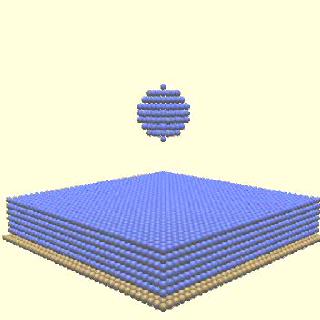
12 Length of smoothing kernel vi Fluid particles fixed on solid wall (Wall particles)
13 r = v z g x Lz Lx
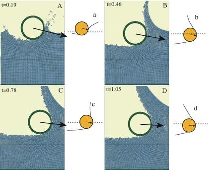
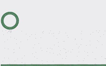
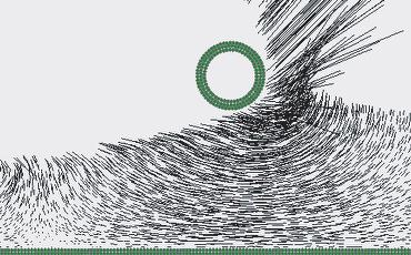
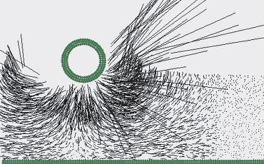
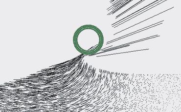
14 円柱と水面の衝突 ー衝突の様子と速度プロファイル 上図a-d; E. G. Richardson, Proc. Phys. Soc. London, Sect. A 6 (948)より引用 年月9日木曜日
15 斜め衝突の間に円柱が受ける力 粒子の初期配置の影響 粒子の配置を正方格子とランダム配置に選んだ二つの結果を比較 force v r.5 force v r Square Lattice Random.6 Square Lattice Random.5.4 fz.3 fz.5.. T=r/cで 時間平均処理 fx -. fx t t r/v r/v 境界(底面)の影響 深さの異なる水槽 用いたシミュレーションの結果.4 force.3 v r fz Lz=7r Lz=4r fz fx. fz. fx -. fx t r/v 年月9日木曜日 6 7 8
16 θ c tank size lx=3r, lz=4r lx=4r, lz=8r θ c = 8/ σ Critical Angle [deg.] -.5. Specific gravity
17 v

18 5cm θ =.5, φ =, ω = 6[rounds/sec.]

19 5cm θ =.5, φ =, ω = [rounds/sec.]
20 v Minimum Velocity [m/sec.] Experiment SPH Incident Angle [deg.] Experiment SPH Tilt Angle [deg.]
21 v θ =8. φ =
22 z φ = const. p ρ(v n). z' f R x = const. f = pnds = disk s face g C D ρ(v n) n/ds disk s face = C Dρ(v n) Sn d v Water x'

23 衝突のODEモデル 1 無次元化した運動方程式 x z = sin φ F = κs(z )z cos φ F! z (x,z) v F = gr f x R = const. CD Rρ κ= πdρ! g z' xz座標系 v d 円盤下側の角の位置 フロード数 #! "! " "!!!! z z π z + S(z! ) = arcsin + + sin φ sin φ sin φ 流体にひたっている面積 年月9日木曜日 x' Water
24 ODEモデルと SPHシミュレーションの比較 定数κの決定 κ=.94, (Fitting parameter) 円板の受ける力 円板の軌道.6.35 fz fx.3.5. z/r fx -.5 年月9日木曜日.5 -. SPH ODE time r/v.5 ODE SPH.5 fz x/r
25 Minimum Velocity vmin [m/sec.] Criterion A Experiment SPH Theory Tilt Angle [deg.] Incident Angle [deg.] Experiment SPH Theory Tilt Angle [deg.]
26 衝突のODEモデル 解析解 反発 の定義 通常は 水面の高さを基準 にとる 位置条件 ここでは 重力方向の速度を基準にとる 速度条件 円盤の重力方向の速度が反転したら 反発が 起こったものと 見なす x (a) z (b) (c) (d) 年月9日木曜日 = sin φ F = κs(z )z cos φ F! 変曲点の存在条件をしらべる 球と水面の衝突の実験で得られた 衝突後の球の軌道 E. G. Richardson, Proc. Phys. Soc. London, Sect. A 6 (948)
27 v min = θ max = arccos gr cos(θ + φ) F { x sin φ + ( x sin φ + σd cos φ C D R sin φ } ) σd cos φ C D R sin φ φ Minimum Velocity vmin [m/sec.] Experiment SPH Theory Tilt Angle [deg.] Incident Angle [deg.] Experiment SPH Theory Tilt Angle [deg.]
28 35 3 σ. Angle [deg.] Experiment SPH Theory Incident Angle [deg.]
29 Incident speed [m/sec.] n > 38 n > 3 n > n > n > 5 θ Angle of incidence [deg.] Angle of incidence [deg.] 4 3 n > 3 n > 38 v 5[m/sec.] n > n > n > Tilt angle [deg.]
30
 (b) K. Okumura et.")
 高圧の物理学の実験 自由表面を持つ様々な現象への 数値的なアプローチ 円形跳水の問題 Clive Ellegaard")
31 シミュレーション法の応用分野と 今後の課題 濡れ を伴う粉体系へのシミュレーション法の開発 地盤の液状化現象への応用 R+X 非常に大きな変形をともなう粘弾性体 のシミュレーション ゲルの衝突 水滴の衝突 R+X h h (a) (b) K. Okumura et. al. Europhys. Lett. 6, 37 (3) 高圧の物理学の実験 自由表面を持つ様々な現象への 数値的なアプローチ 円形跳水の問題 Clive Ellegaard et. al., Nonlinearity,, (999) Nature, 39, 3 (998) 年月9日木曜日
II ( ) (7/31) II ( [ (3.4)] Navier Stokes [ (6/29)] Navier Stokes 3 [ (6/19)] Re
![II ( ) (7/31) II ( [ (3.4)] Navier Stokes [ (6/29)] Navier Stokes 3 [ (6/19)] Re](/thumbs/94/118770263.jpg "II ( ) (7/31) II ( [ (3.4)] Navier Stokes [ (6/29)] Navier Stokes 3 [ (6/19)] Re") II 29 7 29-7-27 ( ) (7/31) II (http://www.damp.tottori-u.ac.jp/~ooshida/edu/fluid/) [ (3.4)] Navier Stokes [ (6/29)] Navier Stokes 3 [ (6/19)] Reynolds [ (4.6), (45.8)] [ p.186] Navier Stokes I Euler Navier
II 29 7 29-7-27 ( ) (7/31) II (http://www.damp.tottori-u.ac.jp/~ooshida/edu/fluid/) [ (3.4)] Navier Stokes [ (6/29)] Navier Stokes 3 [ (6/19)] Reynolds [ (4.6), (45.8)] [ p.186] Navier Stokes I Euler Navier
A
 A04-164 2008 2 13 1 4 1.1.......................................... 4 1.2..................................... 4 1.3..................................... 4 1.4..................................... 5 2
Untitled
 II 14 14-7-8 8/4 II (http://www.damp.tottori-u.ac.jp/~ooshida/edu/fluid/) [ (3.4)] Navier Stokes [ 6/ ] Navier Stokes 3 [ ] Reynolds [ (4.6), (45.8)] [ p.186] Navier Stokes I 1 balance law t (ρv i )+ j
A Precise Calculation Method of the Gradient Operator in Numerical Computation with the MPS Tsunakiyo IRIBE and Eizo NAKAZA A highly precise numerical
 A Precise Calculation Method of the Gradient Operator in Numerical Computation with the MPS Tsunakiyo IRIBE and Eizo NAKAZA A highly precise numerical calculation method of the gradient as a differential
1 (Berry,1975) 2-6 p (S πr 2 )p πr 2 p 2πRγ p p = 2γ R (2.5).1-1 : : : : ( ).2 α, β α, β () X S = X X α X β (.1) 1 2
 2-6 p (S πr 2 )p πr 2 p 2πRγ p p = 2γ R (2.5).1-1 : : : : ( ).2 α, β α, β () X S = X X α X β (.1) 1 2") 2005 9/8-11 2 2.2 ( 2-5) γ ( ) γ cos θ 2πr πρhr 2 g h = 2γ cos θ ρgr (2.1) γ = ρgrh (2.2) 2 cos θ θ cos θ = 1 (2.2) γ = 1 ρgrh (2.) 2 2. p p ρgh p ( ) p p = p ρgh (2.) h p p = 2γ r 1 1 (Berry,1975) 2-6
2005 9/8-11 2 2.2 ( 2-5) γ ( ) γ cos θ 2πr πρhr 2 g h = 2γ cos θ ρgr (2.1) γ = ρgrh (2.2) 2 cos θ θ cos θ = 1 (2.2) γ = 1 ρgrh (2.) 2 2. p p ρgh p ( ) p p = p ρgh (2.) h p p = 2γ r 1 1 (Berry,1975) 2-6
知能科学:ニューラルネットワーク
 2 3 4 (Neural Network) (Deep Learning) (Deep Learning) ( x x = ax + b x x x ? x x x w σ b = σ(wx + b) x w b w b .2.8.6 σ(x) = + e x.4.2 -.2 - -5 5 x w x2 w2 σ x3 w3 b = σ(w x + w 2 x 2 + w 3 x 3 + b) x,
知能科学:ニューラルネットワーク
 2 3 4 (Neural Network) (Deep Learning) (Deep Learning) ( x x = ax + b x x x ? x x x w σ b = σ(wx + b) x w b w b .2.8.6 σ(x) = + e x.4.2 -.2 - -5 5 x w x2 w2 σ x3 w3 b = σ(w x + w 2 x 2 + w 3 x 3 + b) x,
tomocci ,. :,,,, Lie,,,, Einstein, Newton. 1 M n C. s, M p. M f, p d ds f = dxµ p ds µ f p, X p = X µ µ p = dxµ ds µ p. µ, X µ.,. p,. T M p.
 tomocci 18 7 5...,. :,,,, Lie,,,, Einstein, Newton. 1 M n C. s, M p. M f, p d ds f = dxµ p ds µ f p, X p = X µ µ p = dxµ ds µ p. µ, X µ.,. p,. T M p. M F (M), X(F (M)).. T M p e i = e µ i µ. a a = a i
/ Christopher Essex Radiation and the Violation of Bilinearity in the Thermodynamics of Irreversible Processes, Planet.Space Sci.32 (1984) 1035 Radiat
 1035 Radiat") / Christopher Essex Radiation and the Violation of Bilinearity in the Thermodynamics of Irreversible Processes, Planet.Space Sci.32 (1984) 1035 Radiation and the Continuing Failure of the Bilinear Formalism,
/ Christopher Essex Radiation and the Violation of Bilinearity in the Thermodynamics of Irreversible Processes, Planet.Space Sci.32 (1984) 1035 Radiation and the Continuing Failure of the Bilinear Formalism,
量子力学 問題
 3 : 203 : 0. H = 0 0 2 6 0 () = 6, 2 = 2, 3 = 3 3 H 6 2 3 ϵ,2,3 (2) ψ = (, 2, 3 ) ψ Hψ H (3) P i = i i P P 2 = P 2 P 3 = P 3 P = O, P 2 i = P i (4) P + P 2 + P 3 = E 3 (5) i ϵ ip i H 0 0 (6) R = 0 0 [H,
医系の統計入門第 2 版 サンプルページ この本の定価 判型などは, 以下の URL からご覧いただけます. このサンプルページの内容は, 第 2 版 1 刷発行時のものです.
 医系の統計入門第 2 版 サンプルページ この本の定価 判型などは, 以下の URL からご覧いただけます. http://www.morikita.co.jp/books/mid/009192 このサンプルページの内容は, 第 2 版 1 刷発行時のものです. i 2 t 1. 2. 3 2 3. 6 4. 7 5. n 2 ν 6. 2 7. 2003 ii 2 2013 10 iii 1987
Gmech08.dvi
 51 5 5.1 5.1.1 P r P z θ P P P z e r e, z ) r, θ, ) 5.1 z r e θ,, z r, θ, = r sin θ cos = r sin θ sin 5.1) e θ e z = r cos θ r, θ, 5.1: 0 r
64 3 g=9.85 m/s 2 g=9.791 m/s 2 36, km ( ) 1 () 2 () m/s : : a) b) kg/m kg/m k
 1 () 2 () m/s : : a) b) kg/m kg/m k") 63 3 Section 3.1 g 3.1 3.1: : 64 3 g=9.85 m/s 2 g=9.791 m/s 2 36, km ( ) 1 () 2 () 3 9.8 m/s 2 3.2 3.2: : a) b) 5 15 4 1 1. 1 3 14. 1 3 kg/m 3 2 3.3 1 3 5.8 1 3 kg/m 3 3 2.65 1 3 kg/m 3 4 6 m 3.1. 65 5
63 3 Section 3.1 g 3.1 3.1: : 64 3 g=9.85 m/s 2 g=9.791 m/s 2 36, km ( ) 1 () 2 () 3 9.8 m/s 2 3.2 3.2: : a) b) 5 15 4 1 1. 1 3 14. 1 3 kg/m 3 2 3.3 1 3 5.8 1 3 kg/m 3 3 2.65 1 3 kg/m 3 4 6 m 3.1. 65 5
PowerPoint プレゼンテーション
 米田 戸倉川月 7 限 193~21 西 5-19 応用数学 A 積分定理 Gaussの定理 divbd = B nds Stokesの定理 E bds = E dr Green の定理 g x f y dxdy = fdx + gdy = f e i + ge j dr Gauss の発散定理 S n FdS = Fd 1777-1855 ドイツ Johann arl Friedrich Gauss
untitled
 SPring-8 RFgun JASRI/SPring-8 6..7 Contents.. 3.. 5. 6. 7. 8. . 3 cavity γ E A = er 3 πε γ vb r B = v E c r c A B A ( ) F = e E + v B A A A A B dp e( v B+ E) = = m d dt dt ( γ v) dv e ( ) dt v B E v E
(5) 75 (a) (b) ( 1 ) v ( 1 ) E E 1 v (a) ( 1 ) x E E (b) (a) (b)
 75 (a) (b) ( 1 ) v ( 1 ) E E 1 v (a) ( 1 ) x E E (b) (a) (b)") (5) 74 Re, bondar laer (Prandtl) Re z ω z = x (5) 75 (a) (b) ( 1 ) v ( 1 ) E E 1 v (a) ( 1 ) x E E (b) (a) (b) (5) 76 l V x ) 1/ 1 ( 1 1 1 δ δ = x Re x p V x t V l l (1-1) 1/ 1 δ δ δ δ = x Re p V x t V
(5) 74 Re, bondar laer (Prandtl) Re z ω z = x (5) 75 (a) (b) ( 1 ) v ( 1 ) E E 1 v (a) ( 1 ) x E E (b) (a) (b) (5) 76 l V x ) 1/ 1 ( 1 1 1 δ δ = x Re x p V x t V l l (1-1) 1/ 1 δ δ δ δ = x Re p V x t V
1. z dr er r sinθ dϕ eϕ r dθ eθ dr θ dr dθ r x 0 ϕ r sinθ dϕ r sinθ dϕ y dr dr er r dθ eθ r sinθ dϕ eϕ 2. (r, θ, φ) 2 dr 1 h r dr 1 e r h θ dθ 1 e θ h
 2 dr 1 h r dr 1 e r h θ dθ 1 e θ h") IB IIA 1 1 r, θ, φ 1 (r, θ, φ)., r, θ, φ 0 r
IB IIA 1 1 r, θ, φ 1 (r, θ, φ)., r, θ, φ 0 r
I-2 (100 ) (1) y(x) y dy dx y d2 y dx 2 (a) y + 2y 3y = 9e 2x (b) x 2 y 6y = 5x 4 (2) Bernoulli B n (n = 0, 1, 2,...) x e x 1 = n=0 B 0 B 1 B 2 (3) co
 (1) y(x) y dy dx y d2 y dx 2 (a) y + 2y 3y = 9e 2x (b) x 2 y 6y = 5x 4 (2) Bernoulli B n (n = 0, 1, 2,...) x e x 1 = n=0 B 0 B 1 B 2 (3) co") 16 I ( ) (1) I-1 I-2 I-3 (2) I-1 ( ) (100 ) 2l x x = 0 y t y(x, t) y(±l, t) = 0 m T g y(x, t) l y(x, t) c = 2 y(x, t) c 2 2 y(x, t) = g (A) t 2 x 2 T/m (1) y 0 (x) y 0 (x) = g c 2 (l2 x 2 ) (B) (2) (1)
16 I ( ) (1) I-1 I-2 I-3 (2) I-1 ( ) (100 ) 2l x x = 0 y t y(x, t) y(±l, t) = 0 m T g y(x, t) l y(x, t) c = 2 y(x, t) c 2 2 y(x, t) = g (A) t 2 x 2 T/m (1) y 0 (x) y 0 (x) = g c 2 (l2 x 2 ) (B) (2) (1)
SPring-8ワークショップ_リガク伊藤
 GI SAXS. X X X X GI-SAXS : Grazing-incidence smallangle X-ray scattering. GI-SAXS GI-SAXS GI-SAXS X X X X X GI-SAXS Q Y : Q Z : Q Y - Q Z CCD Charge-coupled device X X APD Avalanche photo diode - cps 8
#A A A F, F d F P + F P = d P F, F y P F F x A.1 ( α, 0), (α, 0) α > 0) (x, y) (x + α) 2 + y 2, (x α) 2 + y 2 d (x + α)2 + y 2 + (x α) 2 + y 2 =
, (α, 0) α > 0) (x, y) (x + α) 2 + y 2, (x α) 2 + y 2 d (x + α)2 + y 2 + (x α) 2 + y 2 =") #A A A. F, F d F P + F P = d P F, F P F F A. α, 0, α, 0 α > 0, + α +, α + d + α + + α + = d d F, F 0 < α < d + α + = d α + + α + = d d α + + α + d α + = d 4 4d α + = d 4 8d + 6 http://mth.cs.kitmi-it.c.jp/
#A A A. F, F d F P + F P = d P F, F P F F A. α, 0, α, 0 α > 0, + α +, α + d + α + + α + = d d F, F 0 < α < d + α + = d α + + α + = d d α + + α + d α + = d 4 4d α + = d 4 8d + 6 http://mth.cs.kitmi-it.c.jp/
1 1. x 1 (1) x 2 + 2x + 5 dx d dx (x2 + 2x + 5) = 2(x + 1) x 1 x 2 + 2x + 5 = x + 1 x 2 + 2x x 2 + 2x + 5 y = x 2 + 2x + 5 dy = 2(x + 1)dx x + 1
 x 2 + 2x + 5 dx d dx (x2 + 2x + 5) = 2(x + 1) x 1 x 2 + 2x + 5 = x + 1 x 2 + 2x x 2 + 2x + 5 y = x 2 + 2x + 5 dy = 2(x + 1)dx x + 1") . ( + + 5 d ( + + 5 ( + + + 5 + + + 5 + + 5 y + + 5 dy ( + + dy + + 5 y log y + C log( + + 5 + C. ++5 (+ +4 y (+/ + + 5 (y + 4 4(y + dy + + 5 dy Arctany+C Arctan + y ( + +C. + + 5 ( + log( + + 5 Arctan
. ( + + 5 d ( + + 5 ( + + + 5 + + + 5 + + 5 y + + 5 dy ( + + dy + + 5 y log y + C log( + + 5 + C. ++5 (+ +4 y (+/ + + 5 (y + 4 4(y + dy + + 5 dy Arctany+C Arctan + y ( + +C. + + 5 ( + log( + + 5 Arctan
Contents 1 Jeans (
 Contents 1 Jeans 2 1.1....................................... 2 1.2................................. 2 1.3............................... 3 2 3 2.1 ( )................................ 4 2.2 WKB........................
66 σ σ (8.1) σ = 0 0 σd = 0 (8.2) (8.2) (8.1) E ρ d = 0... d = 0 (8.3) d 1 NN K K 8.1 d σd σd M = σd = E 2 d (8.4) ρ 2 d = I M = EI ρ 1 ρ = M EI ρ EI
 σ = 0 0 σd = 0 (8.2) (8.2) (8.1) E ρ d = 0... d = 0 (8.3) d 1 NN K K 8.1 d σd σd M = σd = E 2 d (8.4) ρ 2 d = I M = EI ρ 1 ρ = M EI ρ EI") 65 8. K 8 8 7 8 K 6 7 8 K 6 M Q σ (6.4) M O ρ dθ D N d N 1 P Q B C (1 + ε)d M N N h 2 h 1 ( ) B (+) M 8.1: σ = E ρ (E, 1/ρ ) (8.1) 66 σ σ (8.1) σ = 0 0 σd = 0 (8.2) (8.2) (8.1) E ρ d = 0... d = 0 (8.3)
65 8. K 8 8 7 8 K 6 7 8 K 6 M Q σ (6.4) M O ρ dθ D N d N 1 P Q B C (1 + ε)d M N N h 2 h 1 ( ) B (+) M 8.1: σ = E ρ (E, 1/ρ ) (8.1) 66 σ σ (8.1) σ = 0 0 σd = 0 (8.2) (8.2) (8.1) E ρ d = 0... d = 0 (8.3)
.2 ρ dv dt = ρk grad p + 3 η grad (divv) + η 2 v.3 divh = 0, rote + c H t = 0 dive = ρ, H = 0, E = ρ, roth c E t = c ρv E + H c t = 0 H c E t = c ρv T
 + η 2 v.3 divh = 0, rote + c H t = 0 dive = ρ, H = 0, E = ρ, roth c E t = c ρv E + H c t = 0 H c E t = c ρv T") NHK 204 2 0 203 2 24 ( ) 7 00 7 50 203 2 25 ( ) 7 00 7 50 203 2 26 ( ) 7 00 7 50 203 2 27 ( ) 7 00 7 50 I. ( ν R n 2 ) m 2 n m, R = e 2 8πε 0 hca B =.09737 0 7 m ( ν = ) λ a B = 4πε 0ħ 2 m e e 2 = 5.2977
NHK 204 2 0 203 2 24 ( ) 7 00 7 50 203 2 25 ( ) 7 00 7 50 203 2 26 ( ) 7 00 7 50 203 2 27 ( ) 7 00 7 50 I. ( ν R n 2 ) m 2 n m, R = e 2 8πε 0 hca B =.09737 0 7 m ( ν = ) λ a B = 4πε 0ħ 2 m e e 2 = 5.2977
 4 2016 3 8 2.,. 2. Arakawa Jacobin., 2 Adams-Bashforth. Re = 80, 90, 100.. h l, h/l, Kármán, h/l 0.28,, h/l.., (2010), 46.2., t = 100 t = 2000 46.2 < Re 46.5. 1 1 4 2 6 2.1............................
D論研究 :「表面張力対流の基礎的研究」
 D 論研究 : 表面張力対流の基礎的研究 定常 Marangoni 対流 及び非定常 Marangoni 対流に関する実験及び数値解析による検討 Si 単結晶の育成装置 Cz 法による Si 単結晶育成 FZ 法による Si 単結晶育成 気液表面 るつぼ加熱 気液表面 大きな温度差を有す気液表面では表面張力対流 (Marangoni 対流 ) が顕著 プロセス終了後のウエハ Cz 法により育成した
1. ( ) 1.1 t + t [m]{ü(t + t)} + [c]{ u(t + t)} + [k]{u(t + t)} = {f(t + t)} (1) m ü f c u k u 1.2 Newmark β (1) (2) ( [m] + t ) 2 [c] + β( t)2
![1. ( ) 1.1 t + t [m]{ü(t + t)} + [c]{ u(t + t)} + [k]{u(t + t)} = {f(t + t)} (1) m ü f c u k u 1.2 Newmark β (1) (2) ( [m] + t ) 2 [c] + β( t)2](/thumbs/80/80934335.jpg "1. ( ) 1.1 t + t [m]{ü(t + t)} + [c]{ u(t + t)} + [k]{u(t + t)} = {f(t + t)} (1) m ü f c u k u 1.2 Newmark β (1) (2) ( [m] + t ) 2 [c] + β( t)2") 212 1 6 1. (212.8.14) 1 1.1............................................. 1 1.2 Newmark β....................... 1 1.3.................................... 2 1.4 (212.8.19)..................................
212 1 6 1. (212.8.14) 1 1.1............................................. 1 1.2 Newmark β....................... 1 1.3.................................... 2 1.4 (212.8.19)..................................
all.dvi
 72 9 Hooke,,,. Hooke. 9.1 Hooke 1 Hooke. 1, 1 Hooke. σ, ε, Young. σ ε (9.1), Young. τ γ G τ Gγ (9.2) X 1, X 2. Poisson, Poisson ν. ν ε 22 (9.) ε 11 F F X 2 X 1 9.1: Poisson 9.1. Hooke 7 Young Poisson G
ψ(, v = u + v = (5.1 u = ψ, v = ψ (5.2 ψ 2 P P F ig.23 ds d d n P flow v : d/ds = (d/ds, d/ds 9 n=(d/ds, d/ds ds 2 = d 2 d v n P ψ( ψ
 KENZOU 28 8 9 9/6 4 1 2 3 4 2 2 5 2 2 5.1............................................. 2 5.2......................................... 3 5.2.1........................................ 3 5.2.2...............................
() x + y + y + x dy dx = 0 () dy + xy = x dx y + x y ( 5) ( s55906) 0.7. (). 5 (). ( 6) ( s6590) 0.8 m n. 0.9 n n A. ( 6) ( s6590) f A (λ) = det(a λi)
 x + y + y + x dy dx = 0 () dy + xy = x dx y + x y ( 5) ( s55906) 0.7. (). 5 (). ( 6) ( s6590) 0.8 m n. 0.9 n n A. ( 6) ( s6590) f A (λ) = det(a λi)") 0. A A = 4 IC () det A () A () x + y + z = x y z X Y Z = A x y z ( 5) ( s5590) 0. a + b + c b c () a a + b + c c a b a + b + c 0 a b c () a 0 c b b c 0 a c b a 0 0. A A = 7 5 4 5 0 ( 5) ( s5590) () A ()
0. A A = 4 IC () det A () A () x + y + z = x y z X Y Z = A x y z ( 5) ( s5590) 0. a + b + c b c () a a + b + c c a b a + b + c 0 a b c () a 0 c b b c 0 a c b a 0 0. A A = 7 5 4 5 0 ( 5) ( s5590) () A ()
 1 3 1.1.......................... 3 1............................... 3 1.3....................... 5 1.4.......................... 6 1.5........................ 7 8.1......................... 8..............................
1 I 1.1 ± e = = - = C C MKSA [m], [Kg] [s] [A] 1C 1A 1 MKSA 1C 1C +q q +q q 1
![1 I 1.1 ± e = = - = C C MKSA [m], [Kg] [s] [A] 1C 1A 1 MKSA 1C 1C +q q +q q 1](/thumbs/94/121802164.jpg "1 I 1.1 ± e = = - = C C MKSA [m], [Kg] [s] [A] 1C 1A 1 MKSA 1C 1C +q q +q q 1") 1 I 1.1 ± e = = - =1.602 10 19 C C MKA [m], [Kg] [s] [A] 1C 1A 1 MKA 1C 1C +q q +q q 1 1.1 r 1,2 q 1, q 2 r 12 2 q 1, q 2 2 F 12 = k q 1q 2 r 12 2 (1.1) k 2 k 2 ( r 1 r 2 ) ( r 2 r 1 ) q 1 q 2 (q 1 q 2
1 I 1.1 ± e = = - =1.602 10 19 C C MKA [m], [Kg] [s] [A] 1C 1A 1 MKA 1C 1C +q q +q q 1 1.1 r 1,2 q 1, q 2 r 12 2 q 1, q 2 2 F 12 = k q 1q 2 r 12 2 (1.1) k 2 k 2 ( r 1 r 2 ) ( r 2 r 1 ) q 1 q 2 (q 1 q 2
<4D F736F F F696E74202D20836F CC8A C58B858B4F93B982A882E682D1978E89BA814091B28BC68CA48B E >
 バットの角度 打球軌道および落下地点の関係 T999 和田真迪 担当教員 飯田晋司 目次 1. はじめに. ボールとバットの衝突 -1 座標系 -ボールとバットの衝突の前後でのボールの速度 3. ボールの軌道の計算 4. おわりに参考文献 はじめに この研究テーマにした理由は 好きな野球での小さい頃からの疑問であるバッテングについて 角度が変わればどう打球に変化が起こるのかが大学で学んだ物理と数学んだ物理と数学を使って判明できると思ったから
4 2 Rutherford 89 Rydberg λ = R ( n 2 ) n 2 n = n +,n +2, n = Lyman n =2 Balmer n =3 Paschen R Rydberg R = cm 896 Zeeman Zeeman Zeeman Lorentz
 n 2 n = n +,n +2, n = Lyman n =2 Balmer n =3 Paschen R Rydberg R = cm 896 Zeeman Zeeman Zeeman Lorentz") 2 Rutherford 2. Rutherford N. Bohr Rutherford 859 Kirchhoff Bunsen 86 Maxwell Maxwell 885 Balmer λ Balmer λ = 364.56 n 2 n 2 4 Lyman, Paschen 3 nm, n =3, 4, 5, 4 2 Rutherford 89 Rydberg λ = R ( n 2 ) n
2 Rutherford 2. Rutherford N. Bohr Rutherford 859 Kirchhoff Bunsen 86 Maxwell Maxwell 885 Balmer λ Balmer λ = 364.56 n 2 n 2 4 Lyman, Paschen 3 nm, n =3, 4, 5, 4 2 Rutherford 89 Rydberg λ = R ( n 2 ) n
chap03.dvi
 99 3 (Coriolis) cm m (free surface wave) 3.1 Φ 2.5 (2.25) Φ 100 3 r =(x, y, z) x y z F (x, y, z, t) =0 ( DF ) Dt = t + Φ F =0 onf =0. (3.1) n = F/ F (3.1) F n Φ = Φ n = 1 F F t Vn on F = 0 (3.2) Φ (3.1)
修士論文
 SAW 14 2 M3622 i 1 1 1-1 1 1-2 2 1-3 2 2 3 2-1 3 2-2 5 2-3 7 2-3-1 7 2-3-2 2-3-3 SAW 12 3 13 3-1 13 3-2 14 4 SAW 19 4-1 19 4-2 21 4-2-1 21 4-2-2 22 4-3 24 4-4 35 5 SAW 36 5-1 Wedge 36 5-1-1 SAW 36 5-1-2
A 99% MS-Free Presentation
 A 99% MS-Free Presentation 2 Galactic Dynamics (Binney & Tremaine 1987, 2008) Dynamics of Galaxies (Bertin 2000) Dynamical Evolution of Globular Clusters (Spitzer 1987) The Gravitational Million-Body Problem
(1.2) T D = 0 T = D = 30 kn 1.2 (1.4) 2F W = 0 F = W/2 = 300 kn/2 = 150 kn 1.3 (1.9) R = W 1 + W 2 = = 1100 N. (1.9) W 2 b W 1 a = 0
 T D = 0 T = D = 30 kn 1.2 (1.4) 2F W = 0 F = W/2 = 300 kn/2 = 150 kn 1.3 (1.9) R = W 1 + W 2 = = 1100 N. (1.9) W 2 b W 1 a = 0") 1 1 1.1 1.) T D = T = D = kn 1. 1.4) F W = F = W/ = kn/ = 15 kn 1. 1.9) R = W 1 + W = 6 + 5 = 11 N. 1.9) W b W 1 a = a = W /W 1 )b = 5/6) = 5 cm 1.4 AB AC P 1, P x, y x, y y x 1.4.) P sin 6 + P 1 sin 45
1 1 1.1 1.) T D = T = D = kn 1. 1.4) F W = F = W/ = kn/ = 15 kn 1. 1.9) R = W 1 + W = 6 + 5 = 11 N. 1.9) W b W 1 a = a = W /W 1 )b = 5/6) = 5 cm 1.4 AB AC P 1, P x, y x, y y x 1.4.) P sin 6 + P 1 sin 45
微分積分 サンプルページ この本の定価 判型などは, 以下の URL からご覧いただけます. このサンプルページの内容は, 初版 1 刷発行時のものです.
 微分積分 サンプルページ この本の定価 判型などは, 以下の URL からご覧いただけます. ttp://www.morikita.co.jp/books/mid/00571 このサンプルページの内容は, 初版 1 刷発行時のものです. i ii 014 10 iii [note] 1 3 iv 4 5 3 6 4 x 0 sin x x 1 5 6 z = f(x, y) 1 y = f(x)
A (1) = 4 A( 1, 4) 1 A 4 () = tan A(0, 0) π A π
 = 4 A( 1, 4) 1 A 4 () = tan A(0, 0) π A π") 4 4.1 4.1.1 A = f() = f() = a f (a) = f() (a, f(a)) = f() (a, f(a)) f(a) = f 0 (a)( a) 4.1 (4, ) = f() = f () = 1 = f (4) = 1 4 4 (4, ) = 1 ( 4) 4 = 1 4 + 1 17 18 4 4.1 A (1) = 4 A( 1, 4) 1 A 4 () = tan
4 4.1 4.1.1 A = f() = f() = a f (a) = f() (a, f(a)) = f() (a, f(a)) f(a) = f 0 (a)( a) 4.1 (4, ) = f() = f () = 1 = f (4) = 1 4 4 (4, ) = 1 ( 4) 4 = 1 4 + 1 17 18 4 4.1 A (1) = 4 A( 1, 4) 1 A 4 () = tan
 B 1 B.1.......................... 1 B.1.1................. 1 B.1.2................. 2 B.2........................... 5 B.2.1.......................... 5 B.2.2.................. 6 B.2.3..................
Venkatram and Wyngaard, Lectures on Air Pollution Modeling, m km 6.2 Stull, An Introduction to Boundary Layer Meteorology,
 65 6 6.1 No.4 1982 1 1981 J. C. Kaimal 1993 1994 Turbulence and Diffusion in the Atmosphere : Lectures in Environmental Sciences, by A. K. Blackadar, Springer, 1998 An Introduction to Boundary Layer Meteorology,
sec13.dvi
 13 13.1 O r F R = m d 2 r dt 2 m r m = F = m r M M d2 R dt 2 = m d 2 r dt 2 = F = F (13.1) F O L = r p = m r ṙ dl dt = m ṙ ṙ + m r r = r (m r ) = r F N. (13.2) N N = R F 13.2 O ˆn ω L O r u u = ω r 1 1:
t = h x z z = h z = t (x, z) (v x (x, z, t), v z (x, z, t)) ρ v x x + v z z = 0 (1) 2-2. (v x, v z ) φ(x, z, t) v x = φ x, v z
 (v x (x, z, t), v z (x, z, t)) ρ v x x + v z z = 0 (1) 2-2. (v x, v z ) φ(x, z, t) v x = φ x, v z") I 1 m 2 l k 2 x = 0 x 1 x 1 2 x 2 g x x 2 x 1 m k m 1-1. L x 1, x 2, ẋ 1, ẋ 2 ẋ 1 x = 0 1-2. 2 Q = x 1 + x 2 2 q = x 2 x 1 l L Q, q, Q, q M = 2m µ = m 2 1-3. Q q 1-4. 2 x 2 = h 1 x 1 t = 0 2 1 t x 1 (t)
I 1 m 2 l k 2 x = 0 x 1 x 1 2 x 2 g x x 2 x 1 m k m 1-1. L x 1, x 2, ẋ 1, ẋ 2 ẋ 1 x = 0 1-2. 2 Q = x 1 + x 2 2 q = x 2 x 1 l L Q, q, Q, q M = 2m µ = m 2 1-3. Q q 1-4. 2 x 2 = h 1 x 1 t = 0 2 1 t x 1 (t)
5 1.2, 2, d a V a = M (1.2.1), M, a,,,,, Ω, V a V, V a = V + Ω r. (1.2.2), r i 1, i 2, i 3, i 1, i 2, i 3, A 2, A = 3 A n i n = n=1 da = 3 = n=1 3 n=1
, M, a,,,,, Ω, V a V, V a = V + Ω r. (1.2.2), r i 1, i 2, i 3, i 1, i 2, i 3, A 2, A = 3 A n i n = n=1 da = 3 = n=1 3 n=1") 4 1 1.1 ( ) 5 1.2, 2, d a V a = M (1.2.1), M, a,,,,, Ω, V a V, V a = V + Ω r. (1.2.2), r i 1, i 2, i 3, i 1, i 2, i 3, A 2, A = 3 A n i n = n=1 da = 3 = n=1 3 n=1 da n i n da n i n + 3 A ni n n=1 3 n=1
4 1 1.1 ( ) 5 1.2, 2, d a V a = M (1.2.1), M, a,,,,, Ω, V a V, V a = V + Ω r. (1.2.2), r i 1, i 2, i 3, i 1, i 2, i 3, A 2, A = 3 A n i n = n=1 da = 3 = n=1 3 n=1 da n i n da n i n + 3 A ni n n=1 3 n=1
 211 kotaro@math.titech.ac.jp 1 R *1 n n R n *2 R n = {(x 1,..., x n ) x 1,..., x n R}. R R 2 R 3 R n R n R n D D R n *3 ) (x 1,..., x n ) f(x 1,..., x n ) f D *4 n 2 n = 1 ( ) 1 f D R n f : D R 1.1. (x,
重力方向に基づくコントローラの向き決定方法
 ( ) 2/Sep 09 1 ( ) ( ) 3 2 X w, Y w, Z w +X w = +Y w = +Z w = 1 X c, Y c, Z c X c, Y c, Z c X w, Y w, Z w Y c Z c X c 1: X c, Y c, Z c Kentaro Yamaguchi@bandainamcogames.co.jp 1 M M v 0, v 1, v 2 v 0 v
Part () () Γ Part ,
 () Γ Part ,") Contents a 6 6 6 6 6 6 6 7 7. 8.. 8.. 8.3. 8 Part. 9. 9.. 9.. 3. 3.. 3.. 3 4. 5 4.. 5 4.. 9 4.3. 3 Part. 6 5. () 6 5.. () 7 5.. 9 5.3. Γ 3 6. 3 6.. 3 6.. 3 6.3. 33 Part 3. 34 7. 34 7.. 34 7.. 34 8. 35
Contents a 6 6 6 6 6 6 6 7 7. 8.. 8.. 8.3. 8 Part. 9. 9.. 9.. 3. 3.. 3.. 3 4. 5 4.. 5 4.. 9 4.3. 3 Part. 6 5. () 6 5.. () 7 5.. 9 5.3. Γ 3 6. 3 6.. 3 6.. 3 6.3. 33 Part 3. 34 7. 34 7.. 34 7.. 34 8. 35
D v D F v/d F v D F η v D (3.2) (a) F=0 (b) v=const. D F v Newtonian fluid σ ė σ = ηė (2.2) ė kl σ ij = D ijkl ė kl D ijkl (2.14) ė ij (3.3) µ η visco
 (a) F=0 (b) v=const. D F v Newtonian fluid σ ė σ = ηė (2.2) ė kl σ ij = D ijkl ė kl D ijkl (2.14) ė ij (3.3) µ η visco") post glacial rebound 3.1 Viscosity and Newtonian fluid f i = kx i σ ij e kl ideal fluid (1.9) irreversible process e ij u k strain rate tensor (3.1) v i u i / t e ij v F 23 D v D F v/d F v D F η v D (3.2)
post glacial rebound 3.1 Viscosity and Newtonian fluid f i = kx i σ ij e kl ideal fluid (1.9) irreversible process e ij u k strain rate tensor (3.1) v i u i / t e ij v F 23 D v D F v/d F v D F η v D (3.2)
Note.tex 2008/09/19( )
") 1 20 9 19 2 1 5 1.1........................ 5 1.2............................. 8 2 9 2.1............................. 9 2.2.............................. 10 3 13 3.1.............................. 13 3.2..................................
1 20 9 19 2 1 5 1.1........................ 5 1.2............................. 8 2 9 2.1............................. 9 2.2.............................. 10 3 13 3.1.............................. 13 3.2..................................
 n ξ n,i, i = 1,, n S n ξ n,i n 0 R 1,.. σ 1 σ i .10.14.15 0 1 0 1 1 3.14 3.18 3.19 3.14 3.14,. ii 1 1 1.1..................................... 1 1............................... 3 1.3.........................
vol5-honma (LSR: Local Standard of Rest) 2.1 LSR R 0 LSR Θ 0 (Galactic Constant) 1985 (IAU: International Astronomical Union) R 0 =8.5
 2.1 LSR R 0 LSR Θ 0 (Galactic Constant) 1985 (IAU: International Astronomical Union) R 0 =8.5") 2.2 1 2.2 2.2.1 (LSR: Local Standard of Rest) 2.1 LSR R 0 LSR Θ 0 (Galactic Constant) 1985 (IAU: International Astronomical Union) R 0 =8.5 kpc, Θ 0 = 220 km s 1. (2.1) R 0 7kpc 8kpc Θ 0 180 km s 1 270
2.2 1 2.2 2.2.1 (LSR: Local Standard of Rest) 2.1 LSR R 0 LSR Θ 0 (Galactic Constant) 1985 (IAU: International Astronomical Union) R 0 =8.5 kpc, Θ 0 = 220 km s 1. (2.1) R 0 7kpc 8kpc Θ 0 180 km s 1 270
No δs δs = r + δr r = δr (3) δs δs = r r = δr + u(r + δr, t) u(r, t) (4) δr = (δx, δy, δz) u i (r + δr, t) u i (r, t) = u i x j δx j (5) δs 2
 δs δs = r r = δr + u(r + δr, t) u(r, t) (4) δr = (δx, δy, δz) u i (r + δr, t) u i (r, t) = u i x j δx j (5) δs 2") No.2 1 2 2 δs δs = r + δr r = δr (3) δs δs = r r = δr + u(r + δr, t) u(r, t) (4) δr = (δx, δy, δz) u i (r + δr, t) u i (r, t) = u i δx j (5) δs 2 = δx i δx i + 2 u i δx i δx j = δs 2 + 2s ij δx i δx j
No.2 1 2 2 δs δs = r + δr r = δr (3) δs δs = r r = δr + u(r + δr, t) u(r, t) (4) δr = (δx, δy, δz) u i (r + δr, t) u i (r, t) = u i δx j (5) δs 2 = δx i δx i + 2 u i δx i δx j = δs 2 + 2s ij δx i δx j
 2007 5 iii 1 1 1.1.................... 1 2 5 2.1 (shear stress) (shear strain)...... 5 2.1.1...................... 6 2.1.2.................... 6 2.2....................... 7 2.2.1........................
JKR Point loading of an elastic half-space 2 3 Pressure applied to a circular region Boussinesq, n =
 JKR 17 9 15 1 Point loading of an elastic half-space Pressure applied to a circular region 4.1 Boussinesq, n = 1.............................. 4. Hertz, n = 1.................................. 6 4 Hertz
IV (2)
") COMPUTATIONAL FLUID DYNAMICS (CFD) IV (2) The Analysis of Numerical Schemes (2) 11. Iterative methods for algebraic systems Reima Iwatsu, e-mail : iwatsu@cck.dendai.ac.jp Winter Semester 2007, Graduate
COMPUTATIONAL FLUID DYNAMICS (CFD) IV (2) The Analysis of Numerical Schemes (2) 11. Iterative methods for algebraic systems Reima Iwatsu, e-mail : iwatsu@cck.dendai.ac.jp Winter Semester 2007, Graduate
I
 I 6 4 10 1 1 1.1............... 1 1................ 1 1.3.................... 1.4............... 1.4.1.............. 1.4................. 1.4.3........... 3 1.4.4.. 3 1.5.......... 3 1.5.1..............
 20 4 20 i 1 1 1.1............................ 1 1.2............................ 4 2 11 2.1................... 11 2.2......................... 11 2.3....................... 19 3 25 3.1.............................
Gauss Gauss ɛ 0 E ds = Q (1) xy σ (x, y, z) (2) a ρ(x, y, z) = x 2 + y 2 (r, θ, φ) (1) xy A Gauss ɛ 0 E ds = ɛ 0 EA Q = ρa ɛ 0 EA = ρea E = (ρ/ɛ 0 )e
 xy σ (x, y, z) (2) a ρ(x, y, z) = x 2 + y 2 (r, θ, φ) (1) xy A Gauss ɛ 0 E ds = ɛ 0 EA Q = ρa ɛ 0 EA = ρea E = (ρ/ɛ 0 )e") 7 -a 7 -a February 4, 2007 1. 2. 3. 4. 1. 2. 3. 1 Gauss Gauss ɛ 0 E ds = Q (1) xy σ (x, y, z) (2) a ρ(x, y, z) = x 2 + y 2 (r, θ, φ) (1) xy A Gauss ɛ 0 E ds = ɛ 0 EA Q = ρa ɛ 0 EA = ρea E = (ρ/ɛ 0 )e z
7 -a 7 -a February 4, 2007 1. 2. 3. 4. 1. 2. 3. 1 Gauss Gauss ɛ 0 E ds = Q (1) xy σ (x, y, z) (2) a ρ(x, y, z) = x 2 + y 2 (r, θ, φ) (1) xy A Gauss ɛ 0 E ds = ɛ 0 EA Q = ρa ɛ 0 EA = ρea E = (ρ/ɛ 0 )e z
: (a) ( ) A (b) B ( ) A B 11.: (a) x,y (b) r,θ (c) A (x) V A B (x + dx) ( ) ( 11.(a)) dv dt = 0 (11.6) r= θ =
 ( ) A (b) B ( ) A B 11.: (a) x,y (b) r,θ (c) A (x) V A B (x + dx) ( ) ( 11.(a)) dv dt = 0 (11.6) r= θ =") 1 11 11.1 ψ e iα ψ, ψ ψe iα (11.1) *1) L = ψ(x)(γ µ i µ m)ψ(x) ) ( ) ψ e iα(x) ψ(x), ψ(x) ψ(x)e iα(x) (11.3) µ µ + iqa µ (x) (11.4) A µ (x) A µ(x) = A µ (x) + 1 q µα(x) (11.5) 11.1.1 ( ) ( 11.1 ) * 1)
1 11 11.1 ψ e iα ψ, ψ ψe iα (11.1) *1) L = ψ(x)(γ µ i µ m)ψ(x) ) ( ) ψ e iα(x) ψ(x), ψ(x) ψ(x)e iα(x) (11.3) µ µ + iqa µ (x) (11.4) A µ (x) A µ(x) = A µ (x) + 1 q µα(x) (11.5) 11.1.1 ( ) ( 11.1 ) * 1)
Gmech08.dvi
 145 13 13.1 13.1.1 0 m mg S 13.1 F 13.1 F /m S F F 13.1 F mg S F F mg 13.1: m d2 r 2 = F + F = 0 (13.1) 146 13 F = F (13.2) S S S S S P r S P r r = r 0 + r (13.3) r 0 S S m d2 r 2 = F (13.4) (13.3) d 2
untitled
 MRR Physical Basis( 1.8.4) METEK MRR 1 MRR 1.1 MRR 24GHz FM-CW(frequency module continuous wave) 30 r+ r f+ f 1.2 1 4 MRR 24GHz 1.3 50mW 1 rf- (waveguide) (horn) 60cm ( monostatic radar) (continuous wave)
2009 I 2 II III 14, 15, α β α β l 0 l l l l γ (1) γ = αβ (2) α β n n cos 2k n n π sin 2k n π k=1 k=1 3. a 0, a 1,..., a n α a
 γ = αβ (2) α β n n cos 2k n n π sin 2k n π k=1 k=1 3. a 0, a 1,..., a n α a") 009 I II III 4, 5, 6 4 30. 0 α β α β l 0 l l l l γ ) γ αβ ) α β. n n cos k n n π sin k n π k k 3. a 0, a,..., a n α a 0 + a x + a x + + a n x n 0 ᾱ 4. [a, b] f y fx) y x 5. ) Arcsin 4) Arccos ) ) Arcsin
009 I II III 4, 5, 6 4 30. 0 α β α β l 0 l l l l γ ) γ αβ ) α β. n n cos k n n π sin k n π k k 3. a 0, a,..., a n α a 0 + a x + a x + + a n x n 0 ᾱ 4. [a, b] f y fx) y x 5. ) Arcsin 4) Arccos ) ) Arcsin
85 4
 85 4 86 Copright c 005 Kumanekosha 4.1 ( ) ( t ) t, t 4.1.1 t Step! (Step 1) (, 0) (Step ) ±V t (, t) I Check! P P V t π 54 t = 0 + V (, t) π θ : = θ : π ) θ = π ± sin ± cos t = 0 (, 0) = sin π V + t +V
19 σ = P/A o σ B Maximum tensile strength σ % 0.2% proof stress σ EL Elastic limit Work hardening coefficient failure necking σ PL Proportional
 19 σ = P/A o σ B Maximum tensile strength σ 0. 0.% 0.% proof stress σ EL Elastic limit Work hardening coefficient failure necking σ PL Proportional limit ε p = 0.% ε e = σ 0. /E plastic strain ε = ε e
6kg 1.1m 1.m.1m.1 l λ ϵ λ l + λ l l l dl dl + dλ ϵ dλ dl dl + dλ dl dl 3 1. JIS 1 6kg 1% 66kg 1 13 σ a1 σ m σ a1 σ m σ m σ a1 f f σ a1 σ a1 σ m f 4
 35-8585 7 8 1 I I 1 1.1 6kg 1m P σ σ P 1 l l λ λ l 1.m 1 6kg 1.1m 1.m.1m.1 l λ ϵ λ l + λ l l l dl dl + dλ ϵ dλ dl dl + dλ dl dl 3 1. JIS 1 6kg 1% 66kg 1 13 σ a1 σ m σ a1 σ m σ m σ a1 f f σ a1 σ a1 σ m
mt_4.dvi
 ( ) 2006 1 PI 1 1 1.1................................. 1 1.2................................... 1 2 2 2.1...................................... 2 2.1.1.......................... 2 2.1.2..............................
Q = va = kia (1.2) 1.2 ( ) 2 ( 1.2) 1.2(a) (1.2) k = Q/iA = Q L/h A (1.3) 1.2(b) t 1 t 2 h 1 h 2 a
 1.2 ( ) 2 ( 1.2) 1.2(a) (1.2) k = Q/iA = Q L/h A (1.3) 1.2(b) t 1 t 2 h 1 h 2 a") 1 1 1.1 (Darcy) v(cm/s) (1.1) v = ki (1.1) v k i 1.1 h ( )L i = h/l 1.1 t 1 h(cm) (t 2 t 1 ) 1.1 A Q(cm 3 /s) 2 1 1.1 Q = va = kia (1.2) 1.2 ( ) 2 ( 1.2) 1.2(a) (1.2) k = Q/iA = Q L/h A (1.3) 1.2(b) t
1 1 1.1 (Darcy) v(cm/s) (1.1) v = ki (1.1) v k i 1.1 h ( )L i = h/l 1.1 t 1 h(cm) (t 2 t 1 ) 1.1 A Q(cm 3 /s) 2 1 1.1 Q = va = kia (1.2) 1.2 ( ) 2 ( 1.2) 1.2(a) (1.2) k = Q/iA = Q L/h A (1.3) 1.2(b) t
1
 GL (a) (b) Ph l P N P h l l Ph Ph Ph Ph l l l l P Ph l P N h l P l .9 αl B βlt D E. 5.5 L r..8 e g s e,e l l W l s l g W W s g l l W W e s g e s g r e l ( s ) l ( l s ) r e l ( s ) l ( l s ) e R e r
A
 A05-132 2010 2 11 1 1 3 1.1.......................................... 3 1.2..................................... 3 1.3..................................... 3 2 4 2.1............................... 4 2.2
DVIOUT-fujin
 2005 Limit Distribution of Quantum Walks and Weyl Equation 2006 3 2 1 2 2 4 2.1...................... 4 2.2......................... 5 2.3..................... 6 3 8 3.1........... 8 3.2..........................
数学の基礎訓練I
 I 9 6 13 1 1 1.1............... 1 1................ 1 1.3.................... 1.4............... 1.4.1.............. 1.4................. 3 1.4.3........... 3 1.4.4.. 3 1.5.......... 3 1.5.1..............
77
 O r r r, F F r,r r = r r F = F (. ) r = r r 76 77 d r = F d r = F (. ) F + F = 0 d ( ) r + r = 0 (. 3) M = + MR = r + r (. 4) P G P MX = + MY = + MZ = z + z PG / PG = / M d R = 0 (. 5) 78 79 d r = F d
* 1 1 (i) (ii) Brückner-Hartree-Fock (iii) (HF, BCS, HFB) (iv) (TDHF,TDHFB) (RPA) (QRPA) (v) (vi) *
 (ii) Brückner-Hartree-Fock (iii) (HF, BCS, HFB) (iv) (TDHF,TDHFB) (RPA) (QRPA) (v) (vi) *") * 1 1 (i) (ii) Brückner-Hartree-Fock (iii) (HF, BCS, HFB) (iv) (TDHF,TDHFB) (RPA) (QRPA) (v) (vi) *1 2004 1 1 ( ) ( ) 1.1 140 MeV 1.2 ( ) ( ) 1.3 2.6 10 8 s 7.6 10 17 s? Λ 2.5 10 10 s 6 10 24 s 1.4 ( m
* 1 1 (i) (ii) Brückner-Hartree-Fock (iii) (HF, BCS, HFB) (iv) (TDHF,TDHFB) (RPA) (QRPA) (v) (vi) *1 2004 1 1 ( ) ( ) 1.1 140 MeV 1.2 ( ) ( ) 1.3 2.6 10 8 s 7.6 10 17 s? Λ 2.5 10 10 s 6 10 24 s 1.4 ( m
ohpr.dvi
 2003-08-04 1984 VP-1001 CPU, 250 MFLOPS, 128 MB 2004ASCI Purple (LLNL)64 CPU 197, 100 TFLOPS, 50 TB, 4.5 MW PC 2 CPU 16, 4 GFLOPS, 32 GB, 3.2 kw 20028 CPU 640, 40 TFLOPS, 10 TB, 10 MW (ASCI: Accelerated
非線形長波モデルと流体粒子法による津波シミュレータの開発 I_ m ρ v p h g a b a 2h b r ab a b Fang W r ab h 5 Wendland 1995 q= r ab /h a d W r ab h
 土木学会論文集 B2( 海岸工学 ) Vol. 70, No. 2, 2014, I_016-I_020 非線形長波モデルと流体粒子法による津波シミュレータの開発 Development of a Tsunami Simulator Integrating the Smoothed-Particle Hydrodynamics Method and the Nonlinear Shallow Water
スライド 1
 非線形数理秋の学校 パターン形成の数理とその周辺 - 反応拡散方程式理論による時 空間パターンの解析を中心に - 2007 年 9 月 25 日 -27 日 モデル方程式を通してみるパターン解析ー進行波からヘリカル波の分岐を例としてー 池田勉 ( 龍谷大学理工学部 ) 講義概要, 講義資料, 講義中に使用する C 言語プログラムと初期値データ, ヘリカル波のアニメーションをウェブで公開しています :
2 Hermite-Gaussian モード 2-1 Hermite-Gaussian モード 自由空間を伝搬するレーザ光は次のような Hermite-gaussian Modes を持つ光波として扱う ことができる ここで U lm (x, y, z) U l (x, z)u m (y, z) e
 U l (x, z)u m (y, z) e") Wavefront Sensor 法による三角共振器のミスアラインメント検出 齊藤高大 新潟大学大学院自然科学研究科電気情報工学専攻博士後期課程 2 年 214 年 8 月 6 日 1 はじめに Input Mode Cleaner(IMC) は Fig.1 に示すような三角共振器である 懸架鏡の共振などにより IMC を構成する各ミラーが角度変化を起こすと 入射光軸と共振器軸との間にずれが生じる
Wavefront Sensor 法による三角共振器のミスアラインメント検出 齊藤高大 新潟大学大学院自然科学研究科電気情報工学専攻博士後期課程 2 年 214 年 8 月 6 日 1 はじめに Input Mode Cleaner(IMC) は Fig.1 に示すような三角共振器である 懸架鏡の共振などにより IMC を構成する各ミラーが角度変化を起こすと 入射光軸と共振器軸との間にずれが生じる
b3e2003.dvi
 15 II 5 5.1 (1) p, q p = (x + 2y, xy, 1), q = (x 2 + 3y 2, xyz, ) (i) p rotq (ii) p gradq D (2) a, b rot(a b) div [11, p.75] (3) (i) f f grad f = 1 2 grad( f 2) (ii) f f gradf 1 2 grad ( f 2) rotf 5.2
2 1 κ c(t) = (x(t), y(t)) ( ) det(c (t), c x (t)) = det (t) x (t) y (t) y = x (t)y (t) x (t)y (t), (t) c (t) = (x (t)) 2 + (y (t)) 2. c (t) =
 = (x(t), y(t)) ( ) det(c (t), c x (t)) = det (t) x (t) y (t) y = x (t)y (t) x (t)y (t), (t) c (t) = (x (t)) 2 + (y (t)) 2. c (t) =") 1 1 1.1 I R 1.1.1 c : I R 2 (i) c C (ii) t I c (t) (0, 0) c (t) c(i) c c(t) 1.1.2 (1) (2) (3) (1) r > 0 c : R R 2 : t (r cos t, r sin t) (2) C f : I R c : I R 2 : t (t, f(t)) (3) y = x c : R R 2 : t (t,
1 1 1.1 I R 1.1.1 c : I R 2 (i) c C (ii) t I c (t) (0, 0) c (t) c(i) c c(t) 1.1.2 (1) (2) (3) (1) r > 0 c : R R 2 : t (r cos t, r sin t) (2) C f : I R c : I R 2 : t (t, f(t)) (3) y = x c : R R 2 : t (t,
6 2 T γ T B (6.4) (6.1) [( d nm + 3 ] 2 nt B )a 3 + nt B da 3 = 0 (6.9) na 3 = T B V 3/2 = T B V γ 1 = const. or T B a 2 = const. (6.10) H 2 = 8π kc2
![6 2 T γ T B (6.4) (6.1) [( d nm + 3 ] 2 nt B )a 3 + nt B da 3 = 0 (6.9) na 3 = T B V 3/2 = T B V γ 1 = const. or T B a 2 = const. (6.10) H 2 = 8π kc2](/thumbs/92/109118076.jpg "6 2 T γ T B (6.4) (6.1) [( d nm + 3 ] 2 nt B )a 3 + nt B da 3 = 0 (6.9) na 3 = T B V 3/2 = T B V γ 1 = const. or T B a 2 = const. (6.10) H 2 = 8π kc2") 1 6 6.1 (??) (P = ρ rad /3) ρ rad T 4 d(ρv ) + PdV = 0 (6.1) dρ rad ρ rad + 4 da a = 0 (6.2) dt T + da a = 0 T 1 a (6.3) ( ) n ρ m = n (m + 12 ) m v2 = n (m + 32 ) T, P = nt (6.4) (6.1) d [(nm + 32 ] )a
1 6 6.1 (??) (P = ρ rad /3) ρ rad T 4 d(ρv ) + PdV = 0 (6.1) dρ rad ρ rad + 4 da a = 0 (6.2) dt T + da a = 0 T 1 a (6.3) ( ) n ρ m = n (m + 12 ) m v2 = n (m + 32 ) T, P = nt (6.4) (6.1) d [(nm + 32 ] )a
QMII_10.dvi
 65 1 1.1 1.1.1 1.1 H H () = E (), (1.1) H ν () = E ν () ν (). (1.) () () = δ, (1.3) μ () ν () = δ(μ ν). (1.4) E E ν () E () H 1.1: H α(t) = c (t) () + dνc ν (t) ν (), (1.5) H () () + dν ν () ν () = 1 (1.6)
KENZOU
 KENZOU 2008 8 9 5 1 2 3 4 2 5 6 2 6.1......................................... 2 6.2......................................... 2 6.3......................................... 4 7 5 8 6 8.1.................................................
II A A441 : October 02, 2014 Version : Kawahira, Tomoki TA (Kondo, Hirotaka )
") II 214-1 : October 2, 214 Version : 1.1 Kawahira, Tomoki TA (Kondo, Hirotaka ) http://www.math.nagoya-u.ac.jp/~kawahira/courses/14w-biseki.html pdf 1 2 1 9 1 16 1 23 1 3 11 6 11 13 11 2 11 27 12 4 12 11
II 214-1 : October 2, 214 Version : 1.1 Kawahira, Tomoki TA (Kondo, Hirotaka ) http://www.math.nagoya-u.ac.jp/~kawahira/courses/14w-biseki.html pdf 1 2 1 9 1 16 1 23 1 3 11 6 11 13 11 2 11 27 12 4 12 11
IPSJ SIG Technical Report Vol.2014-ARC-213 No.24 Vol.2014-HPC-147 No /12/10 GPU 1,a) 1,b) 1,c) 1,d) GPU GPU Structure Of Array Array Of
 1,b) 1,c) 1,d) GPU GPU Structure Of Array Array Of") GPU 1,a) 1,b) 1,c) 1,d) GPU 1 GPU Structure Of Array Array Of Structure 1. MPS(Moving Particle Semi-Implicit) [1] SPH(Smoothed Particle Hydrodynamics) [] DEM(Distinct Element Method)[] [] 1 Tokyo Institute
GPU 1,a) 1,b) 1,c) 1,d) GPU 1 GPU Structure Of Array Array Of Structure 1. MPS(Moving Particle Semi-Implicit) [1] SPH(Smoothed Particle Hydrodynamics) [] DEM(Distinct Element Method)[] [] 1 Tokyo Institute
4‐E ) キュリー温度を利用した消磁:熱消磁
 キュリー温度を利用した消磁:熱消磁") ( ) () x C x = T T c T T c 4D ) ) Fe Ni Fe Fe Ni (Fe Fe Fe Fe Fe 462 Fe76 Ni36 4E ) ) (Fe) 463 4F ) ) ( ) Fe HeNe 17 Fe Fe Fe HeNe 464 Ni Ni Ni HeNe 465 466 (2) Al PtO 2 (liq) 467 4G ) Al 468 Al ( 468
( ) () x C x = T T c T T c 4D ) ) Fe Ni Fe Fe Ni (Fe Fe Fe Fe Fe 462 Fe76 Ni36 4E ) ) (Fe) 463 4F ) ) ( ) Fe HeNe 17 Fe Fe Fe HeNe 464 Ni Ni Ni HeNe 465 466 (2) Al PtO 2 (liq) 467 4G ) Al 468 Al ( 468
: , 2.0, 3.0, 2.0, (%) ( 2.
 ( 2.") 2017 1 2 1.1...................................... 2 1.2......................................... 4 1.3........................................... 10 1.4................................. 14 1.5..........................................
2017 1 2 1.1...................................... 2 1.2......................................... 4 1.3........................................... 10 1.4................................. 14 1.5..........................................
( ) sin 1 x, cos 1 x, tan 1 x sin x, cos x, tan x, arcsin x, arccos x, arctan x. π 2 sin 1 x π 2, 0 cos 1 x π, π 2 < tan 1 x < π 2 1 (1) (
 sin 1 x, cos 1 x, tan 1 x sin x, cos x, tan x, arcsin x, arccos x, arctan x. π 2 sin 1 x π 2, 0 cos 1 x π, π 2 < tan 1 x < π 2 1 (1) (") 6 20 ( ) sin, cos, tan sin, cos, tan, arcsin, arccos, arctan. π 2 sin π 2, 0 cos π, π 2 < tan < π 2 () ( 2 2 lim 2 ( 2 ) ) 2 = 3 sin (2) lim 5 0 = 2 2 0 0 2 2 3 3 4 5 5 2 5 6 3 5 7 4 5 8 4 9 3 4 a 3 b
6 20 ( ) sin, cos, tan sin, cos, tan, arcsin, arccos, arctan. π 2 sin π 2, 0 cos π, π 2 < tan < π 2 () ( 2 2 lim 2 ( 2 ) ) 2 = 3 sin (2) lim 5 0 = 2 2 0 0 2 2 3 3 4 5 5 2 5 6 3 5 7 4 5 8 4 9 3 4 a 3 b
( ) Note (e ) (µ ) (τ ) ( (ν e,e ) e- (ν µ, µ ) µ- (ν τ,τ ) τ- ) ( ) ( ) (SU(2) ) (W +,Z 0,W ) * 1) 3 * 2) [ ] [ ] [ ] ν e ν µ ν τ e
![( ) Note (e ) (µ ) (τ ) ( (ν e,e ) e- (ν µ, µ ) µ- (ν τ,τ ) τ- ) ( ) ( ) (SU(2) ) (W +,Z 0,W ) * 1) 3 * 2) [ ] [ ] [ ] ν e ν µ ν τ e](/thumbs/98/136160482.jpg "( ) Note (e ) (µ ) (τ ) ( (ν e,e ) e- (ν µ, µ ) µ- (ν τ,τ ) τ- ) ( ) ( ) (SU(2) ) (W +,Z 0,W ) * 1) 3 * 2) [ ] [ ] [ ] ν e ν µ ν τ e") ( ) Note 3 19 12 13 8 8.1 (e ) (µ ) (τ ) ( (ν e,e ) e- (ν µ, µ ) µ- (ν τ,τ ) τ- ) ( ) ( ) (SU(2) ) (W +,Z 0,W ) * 1) 3 * 2) [ ] [ ] [ ] ν e ν µ ν τ e µ τ, e R, µ R, τ R (1a) L ( ) ) * 3) W Z 1/2 ( - )
( ) Note 3 19 12 13 8 8.1 (e ) (µ ) (τ ) ( (ν e,e ) e- (ν µ, µ ) µ- (ν τ,τ ) τ- ) ( ) ( ) (SU(2) ) (W +,Z 0,W ) * 1) 3 * 2) [ ] [ ] [ ] ν e ν µ ν τ e µ τ, e R, µ R, τ R (1a) L ( ) ) * 3) W Z 1/2 ( - )
第62巻 第1号 平成24年4月/石こうを用いた木材ペレット
 Bulletin of Japan Association for Fire Science and Engineering Vol. 62. No. 1 (2012) Development of Two-Dimensional Simple Simulation Model and Evaluation of Discharge Ability for Water Discharge of Firefighting
 25 1232052 26 2 5 i 1 1 2 5 2.1................. 5 2.2..................... 6 2.2.1.......................... 6 2.2.2...................... 8 3 9 3.1................................ 9 3.1.1...........
ma22-9 u ( v w) = u v w sin θê = v w sin θ u cos φ = = 2.3 ( a b) ( c d) = ( a c)( b d) ( a d)( b c) ( a b) ( c d) = (a 2 b 3 a 3 b 2 )(c 2 d 3 c 3 d
 = u v w sin θê = v w sin θ u cos φ = = 2.3 ( a b) ( c d) = ( a c)( b d) ( a d)( b c) ( a b) ( c d) = (a 2 b 3 a 3 b 2 )(c 2 d 3 c 3 d") A 2. x F (t) =f sin ωt x(0) = ẋ(0) = 0 ω θ sin θ θ 3! θ3 v = f mω cos ωt x = f mω (t sin ωt) ω t 0 = f ( cos ωt) mω x ma2-2 t ω x f (t mω ω (ωt ) 6 (ωt)3 = f 6m ωt3 2.2 u ( v w) = v ( w u) = w ( u v) ma22-9
A 2. x F (t) =f sin ωt x(0) = ẋ(0) = 0 ω θ sin θ θ 3! θ3 v = f mω cos ωt x = f mω (t sin ωt) ω t 0 = f ( cos ωt) mω x ma2-2 t ω x f (t mω ω (ωt ) 6 (ωt)3 = f 6m ωt3 2.2 u ( v w) = v ( w u) = w ( u v) ma22-9
1. 4cm 16 cm 4cm 20cm 18 cm L λ(x)=ax [kg/m] A x 4cm A 4cm 12 cm h h Y 0 a G 0.38h a b x r(x) x y = 1 h 0.38h G b h X x r(x) 1 S(x) = πr(x) 2 a,b, h,π
![1. 4cm 16 cm 4cm 20cm 18 cm L λ(x)=ax [kg/m] A x 4cm A 4cm 12 cm h h Y 0 a G 0.38h a b x r(x) x y = 1 h 0.38h G b h X x r(x) 1 S(x) = πr(x) 2 a,b, h,π](/thumbs/101/149329485.jpg "1. 4cm 16 cm 4cm 20cm 18 cm L λ(x)=ax [kg/m] A x 4cm A 4cm 12 cm h h Y 0 a G 0.38h a b x r(x) x y = 1 h 0.38h G b h X x r(x) 1 S(x) = πr(x) 2 a,b, h,π") . 4cm 6 cm 4cm cm 8 cm λ()=a [kg/m] A 4cm A 4cm cm h h Y a G.38h a b () y = h.38h G b h X () S() = π() a,b, h,π V = ρ M = ρv G = M h S() 3 d a,b, h 4 G = 5 h a b a b = 6 ω() s v m θ() m v () θ() ω() dθ()
. 4cm 6 cm 4cm cm 8 cm λ()=a [kg/m] A 4cm A 4cm cm h h Y a G.38h a b () y = h.38h G b h X () S() = π() a,b, h,π V = ρ M = ρv G = M h S() 3 d a,b, h 4 G = 5 h a b a b = 6 ω() s v m θ() m v () θ() ω() dθ()
1 (1) () (3) I 0 3 I I d θ = L () dt θ L L θ I d θ = L = κθ (3) dt κ T I T = π κ (4) T I κ κ κ L l a θ L r δr δl L θ ϕ ϕ = rθ (5) l
 () (3) I 0 3 I I d θ = L () dt θ L L θ I d θ = L = κθ (3) dt κ T I T = π κ (4) T I κ κ κ L l a θ L r δr δl L θ ϕ ϕ = rθ (5) l") 1 1 ϕ ϕ ϕ S F F = ϕ (1) S 1: F 1 1 (1) () (3) I 0 3 I I d θ = L () dt θ L L θ I d θ = L = κθ (3) dt κ T I T = π κ (4) T I κ κ κ L l a θ L r δr δl L θ ϕ ϕ = rθ (5) l : l r δr θ πrδr δf (1) (5) δf = ϕ πrδr
1 1 ϕ ϕ ϕ S F F = ϕ (1) S 1: F 1 1 (1) () (3) I 0 3 I I d θ = L () dt θ L L θ I d θ = L = κθ (3) dt κ T I T = π κ (4) T I κ κ κ L l a θ L r δr δl L θ ϕ ϕ = rθ (5) l : l r δr θ πrδr δf (1) (5) δf = ϕ πrδr
 21 2 26 i 1 1 1.1............................ 1 1.2............................ 3 2 9 2.1................... 9 2.2.......... 9 2.3................... 11 2.4....................... 12 3 15 3.1..........
all.dvi
 38 5 Cauchy.,,,,., σ.,, 3,,. 5.1 Cauchy (a) (b) (a) (b) 5.1: 5.1. Cauchy 39 F Q Newton F F F Q F Q 5.2: n n ds df n ( 5.1). df n n df(n) df n, t n. t n = df n (5.1) ds 40 5 Cauchy t l n mds df n 5.3: t
note1.dvi
 (1) 1996 11 7 1 (1) 1. 1 dx dy d x τ xx x x, stress x + dx x τ xx x+dx dyd x x τ xx x dyd y τ xx x τ xx x+dx d dx y x dy 1. dx dy d x τ xy x τ x ρdxdyd x dx dy d ρdxdyd u x t = τ xx x+dx dyd τ xx x dyd
untitled
 (a) (b) (c) (d) Wunderlich 2.5.1 = = =90 2 1 (hkl) {hkl} [hkl] L tan 2θ = r L nλ = 2dsinθ dhkl ( ) = 1 2 2 2 h k l + + a b c c l=2 l=1 l=0 Polanyi nλ = I sinφ I: B A a 110 B c 110 b b 110 µ a 110
(e ) (µ ) (τ ) ( (ν e,e ) e- (ν µ,µ ) µ- (ν τ,τ ) τ- ) ( ) ( ) ( ) (SU(2) ) (W +,Z 0,W ) * 1) [ ] [ ] [ ] ν e ν µ ν τ e µ τ, e R,µ R,τ R (2.1a
![(e ) (µ ) (τ ) ( (ν e,e ) e- (ν µ,µ ) µ- (ν τ,τ ) τ- ) ( ) ( ) ( ) (SU(2) ) (W +,Z 0,W ) * 1) [ ] [ ] [ ] ν e ν µ ν τ e µ τ, e R,µ R,τ R (2.1a](/thumbs/100/144882653.jpg "(e ) (µ ) (τ ) ( (ν e,e ) e- (ν µ,µ ) µ- (ν τ,τ ) τ- ) ( ) ( ) ( ) (SU(2) ) (W +,Z 0,W ) * 1) [ ] [ ] [ ] ν e ν µ ν τ e µ τ, e R,µ R,τ R (2.1a") 1 2 2.1 (e ) (µ ) (τ ) ( (ν e,e ) e- (ν µ,µ ) µ- (ν τ,τ ) τ- ) ( ) ( ) ( ) (SU(2) ) (W +,Z 0,W ) * 1) [ ] [ ] [ ] ν e ν µ ν τ e µ τ, e R,µ R,τ R (2.1a) L ( ) ) * 2) W Z 1/2 ( - ) d u + e + ν e 1 1 0 0
1 2 2.1 (e ) (µ ) (τ ) ( (ν e,e ) e- (ν µ,µ ) µ- (ν τ,τ ) τ- ) ( ) ( ) ( ) (SU(2) ) (W +,Z 0,W ) * 1) [ ] [ ] [ ] ν e ν µ ν τ e µ τ, e R,µ R,τ R (2.1a) L ( ) ) * 2) W Z 1/2 ( - ) d u + e + ν e 1 1 0 0
( ; ) C. H. Scholz, The Mechanics of Earthquakes and Faulting : - ( ) σ = σ t sin 2π(r a) λ dσ d(r a) =
 C. H. Scholz, The Mechanics of Earthquakes and Faulting : - ( ) σ = σ t sin 2π(r a) λ dσ d(r a) =") 1 9 8 1 1 1 ; 1 11 16 C. H. Scholz, The Mechanics of Earthquakes and Faulting 1. 1.1 1.1.1 : - σ = σ t sin πr a λ dσ dr a = E a = π λ σ πr a t cos λ 1 r a/λ 1 cos 1 E: σ t = Eλ πa a λ E/π γ : λ/ 3 γ =
1 9 8 1 1 1 ; 1 11 16 C. H. Scholz, The Mechanics of Earthquakes and Faulting 1. 1.1 1.1.1 : - σ = σ t sin πr a λ dσ dr a = E a = π λ σ πr a t cos λ 1 r a/λ 1 cos 1 E: σ t = Eλ πa a λ E/π γ : λ/ 3 γ =