2014ESJ.key

Size: px

Start display at page:

Download "2014ESJ.key"

あいねえんの
5 years ago
Views:

4 Statistical Software for State Space Models Commandeur et al. (2011) Journal of Statistical Software 41(1)

5 State Space Models in R Petris & Petrone (2011) Journal of Statistical Software 41(4)

8 y t = F t t + v t, v t N (0, V t ) t = G t t 1 + w t, w t N (0, W t ) t = 1,..., n 0 N (m 0, C 0 )

10 ## build function! BuildLLM <- function(theta) {! dlmmodpoly(order = 1,! dv = theta[1],! dw = theta[2])! }

11 ##! fit.llm <- dlmmle(nile, parm = c(100, 2),! build = BuildLLM,! lower = rep(1e-4, 2))!! ## build function! model.llm <- BuildLLM(fit.llm$par)!! ##! smooth.llm <- dlmsmooth(nile, model.llm)

14 #! x <- matrix(c(rep(0, 27),! rep(1, length(nile) - 27)),! ncol = 1)

15 ##! model.reg <- dlmmodreg(x, dw = c(1, 0))! BuildReg <- function(theta) {! V(model.reg) <- exp(theta[1])! diag(w(model.reg))[1] <- exp(theta[2])! return(model.reg)! }

16 ##! fit.reg <- dlmmle(nile,! parm = rep(0, 2),! build = BuildReg)! model.reg <- BuildReg(fit.reg$par)! smooth.reg <- dlmsmooth(nile,! mod = model.reg)

21 y t = Z t t + t, t N (0, H t ) t+1 = T t t + R t t, t N (0, Q t ) t = 1,..., n 1 N (a 1, P 1 )

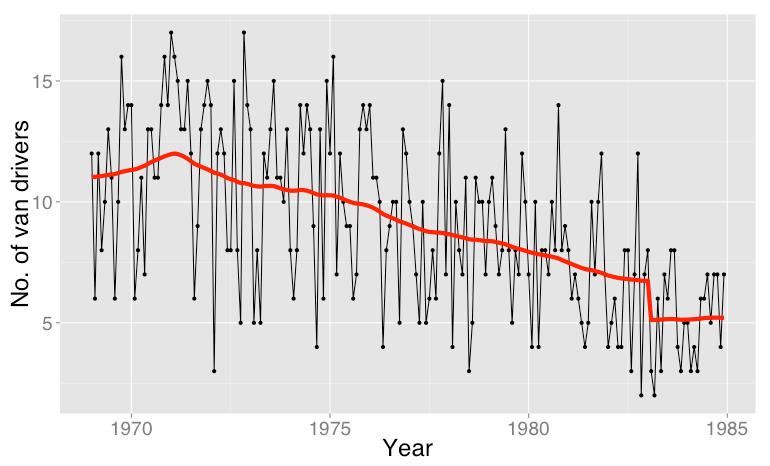
23 model.van <- SSModel(VanKilled ~ law +! SSMtrend(degree = 1,! Q = list(matrix(na))) +! SSMseasonal(period = 12,! sea.type = dummy",! Q = matrix(na)),! data = Seatbelts,! distribution = "poisson")

24 fit.van <- fitssm(inits = c(-4, -7, 2),! model = model.van,! method = BFGS")!! pred.van <- predict(fit.van$model,! states = 1:2)

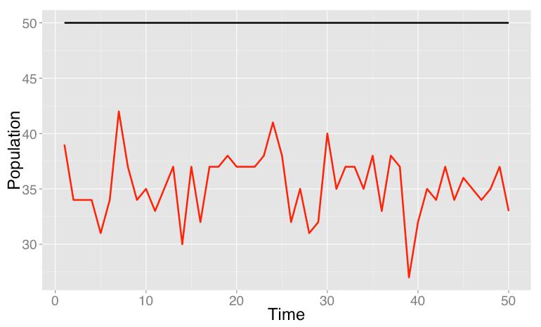
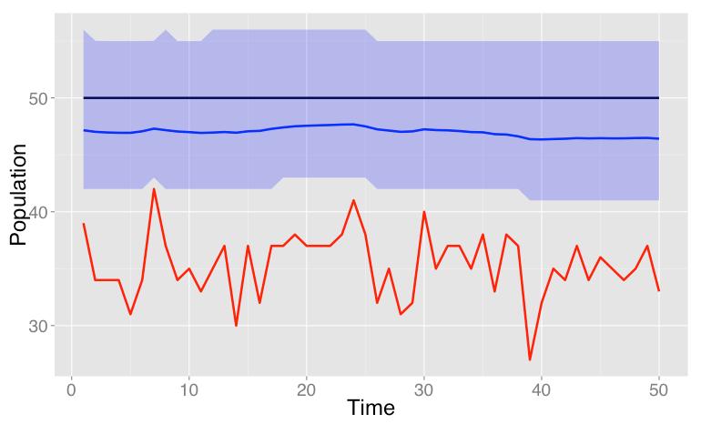
29 set.seed(1234)! n.t <- 50 #! N.lat <- rep(50, n.t) #! p <- 0.7 #! N.obs <- rbinom(n.t, N.lat, p) #!

31 var! N, #! y[n], #! y_hat[n], #! lambda[n], # log(y_hat)! p, #! tau, sigma;

32 model {! ##! for (t in 1:N) {! y[t] ~ dbin(p, y_hat[t]);! y_hat[t] <- trunc(exp(lambda[t]));! }! ##! for (t in 2:N) {! lambda[t] ~ dnorm(lambda[t - 1], tau);! }! ##! lambda[1] ~ dnorm(0, 1.0E-4);! p ~ dbeta(2, 2);! sigma ~ dunif(0, 100);! tau <- 1 / (sigma * sigma);! }

33 inits <- list()! inits[[1]] <- list(p = 0.9, sigma = 1,! lambda = rep(log(max(n.obs) + 1), n.t))! inits[[2]] <- list(p = 0.7, sigma = 3,! lambda = rep(log(max(n.obs) + 1), n.t))! inits[[3]] <- list(p = 0.8, sigma = 5,! lambda = rep(log(max(n.obs) + 1), n.t))!! model <- jags.model("ks51.bug.txt",! data = list(n = n.t, y = N.obs),! inits = inits, n.chains = 3,! n.adapt = )! samp <- coda.samples(model,! variable.names = c("y_hat", sigma",! "p"),! n.iter = , thin = 3000)!

40 data {! int<lower=0> N;! matrix[1, N] y;! }! transformed data {! matrix[1, 1] F;! matrix[1, 1] G;! vector[1] m0;! cov_matrix[1] C0;!! } F[1, 1] <- 1;! G[1, 1] <- 1;! m0[1] <- 0;! C0[1, 1] <- 1.0e+6;!

41 parameters {! real<lower=0> sigma[2];! }! transformed parameters {! vector[1] V;! cov_matrix[1] W;!! V[1] <- sigma[1] * sigma[1];! W[1, 1] <- sigma[2] * sigma[2];! }!

42 model {! y ~ gaussian_dlm_obs(f, G, V, W, m0, C0);! sigma ~ uniform(0, 1.0e+6);! }

43 library(rstan)!! model <- stan("kalman.stan",! data = list(y = matrix(c(nile),! nrow = 1),! N = length(nile)),! pars = c("sigma"),! chains = 3,! iter = 1500, warmup = 500,! thin = 1)

44 traceplot(fit, pars = "sigma", inc_warmup = FALSE)

45 > print(fit)! Inference for Stan model: kalman.! 3 chains, each with iter=1500; warmup=500; thin=1;! post-warmup draws per chain=1000, total post-warmup draws=3000.!! mean se_mean sd 2.5% 25% 50% 75% 97.5% n_eff Rhat! sigma[1] ! sigma[2] ! lp !! Samples were drawn using NUTS(diag_e) at Sun Feb 9 06:06: ! For each parameter, n_eff is a crude measure of effective sample size,! and Rhat is the potential scale reduction factor on split chains (at! convergence, Rhat=1).!

46 sigma <- apply(extract(fit, "sigma")$sigma, 2, mean)!! library(dlm)!! buildnile <- function(theta) {! dlmmodpoly(order = 1, dv = theta[1], dw = theta[2])! }! modnile <- buildnile(sigma^2)! smoothnile <- dlmsmooth(nile, modnile)

49 data {! int<lower=0> N;! real y[n];! }! parameters {! real theta[n];! real<lower=0> sigma[2];! }!

50 model {! //! for (t in 1:N) {! y[t] ~ normal(theta[t], sigma[1]);! }!! //! for (t in 2:N) {! theta[t] ~ normal(theta[t - 1], sigma[2]);! }!! //! theta[1] ~ normal(0, 1.0e+4);! sigma ~ uniform(0, 1.0e+6);! }

@i_kiwamu Bayes - -

Bayes RStan 1 2012 12 1 R @ @i_kiwamu Bayes - - Stan / RStan Bayes Stan Development Team - Andrew Gelman, Bob Carpenter, Matt Hoffman, Ben Goodrich, Michael Malecki, Daniel Lee and Chad Scherrer Open source