ECCS. ECCS,. ( 2. Mac Do-file Editor. Mac Do-file Editor Windows Do-file Editor Top Do-file e
|
|
|
- あいね たみや
- 5 years ago
- Views:
Transcription
1 ECCS. ECCS,. ( 2. Mac Do-file Editor. Mac Do-file Editor Windows Do-file Editor Top Do-file editor, Do View Do-file Editor Execute(do). 3. Mac System Preferences... Display, Resolution Scaled 800x (csv, )

. 2.")
2 2 1 csv File Import Tex data (delimited, *.csv,...) Browse..., csv. xls, xlsx File Import Excel spreadsheet (*.xls, *.xlsx) Excel file: Browse..., xls( xlsx). 1, Import first row as variable names ( ). 2. (Command csv ) (1) pwd (pwd:print working directory),.

3 (2). cd " " (cd:change directory), File Change Working Directory...,. (3) insheet using,., insheet using " " Statistics Summaries, tables, amd tests Summary and descriptive statistics Binomial calculator Sample size n = 865, Successes x = 268 a. a nˆp = = , x = 268. Exact, Wald.
4 :. display 865* cii Binomial Exact -- Variable Obs Mean Std. Err. [95% Conf. Interval] cii , wald (Wald ) -- Binomial Wald --- Variable Obs Mean Std. Err. [95% Conf. Interval] prtesti , count ( 0.31, (count)268 ) One-sample test of proportion x: Number of obs = Variable Mean Std. Err. [95% Conf. Interval] x p = proportion(x) z = Ho: p = 0.4 Ha: p < 0.4 Ha: p!= 0.4 Ha: p > 0.4 Pr(Z < z) = Pr( Z > z ) = Pr(Z > z) = (count), Use integer counts instead of proportions ( ),. 2. Video examples., Video examples, Youtube (, 12). 3. t 0.05 (5%). Command display invttail(, 0.05). display invttail(, 0.05). t, t. Command display ttail(, t ).
5 0.95 (95%). Command display invnormal(0.95). STATA, Command help functions. 4. Data, Other utilities Hand calculator, Create..., Category:. Mac, + Y= \ ( ) (log p t log p t 1 ) 100 (, (log(topix) - log(l.topix))*100 ) , 3 L2.sony, L3.sony , X i = x i Y i E(Y i X i = x i ) = β 0 + β 1 x i 95%, x i 5 Confidence interval for an individual forecast, X i = x i Yi = β 0 + β 1 x i + ϵ i 95%, 95%. ϵ i 1.1:, 95% ( ) 95% ) (1) 95% Confidence Interval 95% Prediction Interval x x 95% CI Fitted values y 95% PI Fitted values y
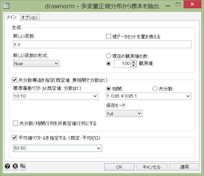
6 :, 95% 95% (2) 95% Confidence Interval & 95% Prediction Interval x 95% PI Fitted values 95% CI y STATA (Data) (Create or change data (Other variable creation commands (Draw sample from normal distribution)
")
7 7 1.1: 1.2: (2)
 (Graphics) ( / )(Twoway graph (scatter, line, etc)) 1.")
8 8 1 (Data) (Data Editor) ( ) (Data Editor (Browse) ( ( )(Data Editor (Edit) (Graphics) ( / )(Twoway graph (scatter, line, etc)) 1.3: (1)
 (Summary")
9 9 1.4: (2) (Data) (Describe data (Summary Statistics (Statistics) / / (Summaries, tables, and tests (Summary and descriptive statistics) (Summary Statistics
,, (Statistics) / / (Summaries, tables, and tests (Summary and")
10 : (1),, (Statistics) / / (Summaries, tables, and tests (Summary and descriptive statistics) (Correlations and covariances 1.7: Command


11 11 1.8: Do-file Editor : Excel Data Editor (2)

12 : 1.13:
) (Browse...), csv. xls, xlsx (File) (Import) Excel (.")
) Excel (Excel file:) (Browse...), xls( xlsx).")
13 13 csv (File) (Import) (,.csv )(Tex data (delimited, *.csv,...)) (Browse...), csv. xls, xlsx (File) (Import) Excel (.xls, xlsx)(excel spreadsheet (*.xls, *.xlsx)) Excel (Excel file:) (Browse...), xls( xlsx). 1, 1 (Import first row as variable names) ( ).
 (Statistics) / / (Summaries, tables, and tests (Classical tests of hypotheses) t ( )(t test (mean-comparison")
14 (Statistics) / / (Summaries, tables, and tests (Summary and descriptive statistics) (Confidence intervals 1.14: 95% ( ) (Statistics) / / (Summaries, tables, and tests (Classical tests of hypotheses) t ( )(t test (mean-comparison test)

15 : : 5% 1.16: : 5%
, (Wald).")
16 16 1 (Statistics) / / (Summaries, tables, and tests (Summary and descriptive statistics) ( )(Binomial calculator) (Sample size) n = 865, (Successes) x = 268 a. a nˆp = = , x = 268. (Exact), (Wald). ( ) (Statistics) / / (Summaries, tables, and tests (Classical tests of hypotheses) ( )(Proportion test calculator


17 : : 5% 1.18: : 5%
 (Time series (Setup and utilities) (Declare dataset to be")
18 (Data) (Create or change data (Create new variable) 1.19: (Statistics) (Time series (Setup and utilities) (Declare dataset to be time-series data)

19 : (Statistics) (Linear models and related (Linear regression)

20 : 1.22: 95% (1)
 21")
21 1.23: 95% (2) 21
Stata11 whitepapers mwp-037 regress - regress regress. regress mpg weight foreign Source SS df MS Number of obs = 74 F(
 mwp-037 regress - regress 1. 1.1 1.2 1.3 2. 3. 4. 5. 1. regress. regress mpg weight foreign Source SS df MS Number of obs = 74 F( 2, 71) = 69.75 Model 1619.2877 2 809.643849 Prob > F = 0.0000 Residual
第2回:データの加工・整理
 2 2018 4 13 1 / 24 1. 2. Excel 3. Stata 4. Stata 5. Stata 2 / 24 1 cross section data e.g., 47 2009 time series data e.g., 1999 2014 5 panel data e.g., 47 1999 2014 5 3 / 24 micro data aggregate data 4
AR(1) y t = φy t 1 + ɛ t, ɛ t N(0, σ 2 ) 1. Mean of y t given y t 1, y t 2, E(y t y t 1, y t 2, ) = φy t 1 2. Variance of y t given y t 1, y t
 y t = φy t 1 + ɛ t, ɛ t N(0, σ 2 ) 1. Mean of y t given y t 1, y t 2, E(y t y t 1, y t 2, ) = φy t 1 2. Variance of y t given y t 1, y t") 87 6.1 AR(1) y t = φy t 1 + ɛ t, ɛ t N(0, σ 2 ) 1. Mean of y t given y t 1, y t 2, E(y t y t 1, y t 2, ) = φy t 1 2. Variance of y t given y t 1, y t 2, V(y t y t 1, y t 2, ) = σ 2 3. Thus, y t y t 1,
87 6.1 AR(1) y t = φy t 1 + ɛ t, ɛ t N(0, σ 2 ) 1. Mean of y t given y t 1, y t 2, E(y t y t 1, y t 2, ) = φy t 1 2. Variance of y t given y t 1, y t 2, V(y t y t 1, y t 2, ) = σ 2 3. Thus, y t y t 1,
Stata 11 Stata ROC whitepaper mwp anova/oneway 3 mwp-042 kwallis Kruskal Wallis 28 mwp-045 ranksum/median / 31 mwp-047 roctab/roccomp ROC 34 mwp-050 s
 BR003 Stata 11 Stata ROC whitepaper mwp anova/oneway 3 mwp-042 kwallis Kruskal Wallis 28 mwp-045 ranksum/median / 31 mwp-047 roctab/roccomp ROC 34 mwp-050 sampsi 47 mwp-044 sdtest 54 mwp-043 signrank/signtest
% 10%, 35%( 1029 ) p (a) 1 p 95% (b) 1 Std. Err. (c) p 40% 5% (d) p 1: STATA (1). prtesti One-sample test of pr
 p (a) 1 p 95% (b) 1 Std. Err. (c) p 40% 5% (d) p 1: STATA (1). prtesti One-sample test of pr") 1 1. 2014 6 2014 6 10 10% 10%, 35%( 1029 ) p (a) 1 p 95% (b) 1 Std. Err. (c) p 40% 5% (d) p 1: STATA (1). prtesti 1029 0.35 0.40 One-sample test of proportion x: Number of obs = 1029 Variable Mean Std.
1 1. 2014 6 2014 6 10 10% 10%, 35%( 1029 ) p (a) 1 p 95% (b) 1 Std. Err. (c) p 40% 5% (d) p 1: STATA (1). prtesti 1029 0.35 0.40 One-sample test of proportion x: Number of obs = 1029 Variable Mean Std.
80 X 1, X 2,, X n ( λ ) λ P(X = x) = f (x; λ) = λx e λ, x = 0, 1, 2, x! l(λ) = n f (x i ; λ) = i=1 i=1 n λ x i e λ i=1 x i! = λ n i=1 x i e nλ n i=1 x
 λ P(X = x) = f (x; λ) = λx e λ, x = 0, 1, 2, x! l(λ) = n f (x i ; λ) = i=1 i=1 n λ x i e λ i=1 x i! = λ n i=1 x i e nλ n i=1 x") 80 X 1, X 2,, X n ( λ ) λ P(X = x) = f (x; λ) = λx e λ, x = 0, 1, 2, x! l(λ) = n f (x i ; λ) = n λ x i e λ x i! = λ n x i e nλ n x i! n n log l(λ) = log(λ) x i nλ log( x i!) log l(λ) λ = 1 λ n x i n =
80 X 1, X 2,, X n ( λ ) λ P(X = x) = f (x; λ) = λx e λ, x = 0, 1, 2, x! l(λ) = n f (x i ; λ) = n λ x i e λ x i! = λ n x i e nλ n x i! n n log l(λ) = log(λ) x i nλ log( x i!) log l(λ) λ = 1 λ n x i n =
Stata 11 Stata ts (ARMA) ARCH/GARCH whitepaper mwp 3 mwp-083 arch ARCH 11 mwp-051 arch postestimation 27 mwp-056 arima ARMA 35 mwp-003 arima postestim
 ARCH/GARCH whitepaper mwp 3 mwp-083 arch ARCH 11 mwp-051 arch postestimation 27 mwp-056 arima ARMA 35 mwp-003 arima postestim") TS001 Stata 11 Stata ts (ARMA) ARCH/GARCH whitepaper mwp 3 mwp-083 arch ARCH 11 mwp-051 arch postestimation 27 mwp-056 arima ARMA 35 mwp-003 arima postestimation 49 mwp-055 corrgram/ac/pac 56 mwp-009 dfgls
TS001 Stata 11 Stata ts (ARMA) ARCH/GARCH whitepaper mwp 3 mwp-083 arch ARCH 11 mwp-051 arch postestimation 27 mwp-056 arima ARMA 35 mwp-003 arima postestimation 49 mwp-055 corrgram/ac/pac 56 mwp-009 dfgls
BR001
 BR001 Stata 11 Stata Stata11 whitepaper mwp 3 mwp-027 22 mwp-028 / 40 mwp-001 logistic/logit 50 mwp-039 logistic/logit postestimation 60 mwp-040 margins 74 mwp-029 regress 90 mwp-037 regress postestimation
第11回:線形回帰モデルのOLS推定
 11 OLS 2018 7 13 1 / 45 1. 2. 3. 2 / 45 n 2 ((y 1, x 1 ), (y 2, x 2 ),, (y n, x n )) linear regression model y i = β 0 + β 1 x i + u i, E(u i x i ) = 0, E(u i u j x i ) = 0 (i j), V(u i x i ) = σ 2, i
Microsoft Word - Text_5_STATA_1_Jp_ doc
 (Blank page) このページを捨てて 次のページから両面してください 社会調査者のための STATA による統計統計データデータ分析 1 < 基礎編 > Text 5 ヒストグラム 平均 分散 標準偏差 対応のある t 検定 ( 事前 - 事後の t 検定 ) 独立の t 検定 (2 群の t 検定 ) Version 2.3 (2013 年 03 月 03 日 ) 佐々木亮 Ph.D. 国際開発センター評価事業部主任研究員立教大学大学院
1 I EViews View Proc Freeze
 EViews 2017 9 6 1 I EViews 4 1 5 2 10 3 13 4 16 4.1 View.......................................... 17 4.2 Proc.......................................... 22 4.3 Freeze & Name....................................
5.2 White
 1 EViews 1 : 2007/5/15 2007/5/25 1 EViews 4 2 ( 6 2.1............................................ 6 2.2 Workfile............................................ 7 2.3 Workfile............................................
こんにちは由美子です
 1 2 . sum Variable Obs Mean Std. Dev. Min Max ---------+----------------------------------------------------- var1 13.4923077.3545926.05 1.1 3 3 3 0.71 3 x 3 C 3 = 0.3579 2 1 0.71 2 x 0.29 x 3 C 2 = 0.4386
k2 ( :35 ) ( k2) (GLM) web web 1 :
 ( k2) (GLM) web web 1 :") 2012 11 01 k2 (2012-10-26 16:35 ) 1 6 2 (2012 11 01 k2) (GLM) kubo@ees.hokudai.ac.jp web http://goo.gl/wijx2 web http://goo.gl/ufq2 1 : 2 2 4 3 7 4 9 5 : 11 5.1................... 13 6 14 6.1......................
2012 11 01 k2 (2012-10-26 16:35 ) 1 6 2 (2012 11 01 k2) (GLM) kubo@ees.hokudai.ac.jp web http://goo.gl/wijx2 web http://goo.gl/ufq2 1 : 2 2 4 3 7 4 9 5 : 11 5.1................... 13 6 14 6.1......................
4.9 Hausman Test Time Fixed Effects Model vs Time Random Effects Model Two-way Fixed Effects Model
 1 EViews 5 2007 7 11 2010 5 17 1 ( ) 3 1.1........................................... 4 1.2................................... 9 2 11 3 14 3.1 Pooled OLS.............................................. 14
4 OLS 4 OLS 4.1 nurseries dual c dual i = c + βnurseries i + ε i (1) 1. OLS Workfile Quick - Estimate Equation OK Equation specification dual c nurser
 1. OLS Workfile Quick - Estimate Equation OK Equation specification dual c nurser") 1 EViews 2 2007/5/17 2007/5/21 4 OLS 2 4.1.............................................. 2 4.2................................................ 9 4.3.............................................. 11 4.4
1 EViews 2 2007/5/17 2007/5/21 4 OLS 2 4.1.............................................. 2 4.2................................................ 9 4.3.............................................. 11 4.4
7 ( 7 ( Workfile Excel hatuden 1000kWh kion_average kion_max kion_min date holiday *1 obon 7.1 Workfile 1. Workfile File - New -
 1 EViews 4 2007 7 4 7 ( 2 7.1 Workfile............................................ 2 7.2........................................... 4 8 6 8.1................................................. 6 8.2................................................
こんにちは由美子です
 Sample size power calculation Sample Size Estimation AZTPIAIDS AIDSAZT AIDSPI AIDSRNA AZTPr (S A ) = π A, PIPr (S B ) = π B AIDS (sampling)(inference) π A, π B π A - π B = 0.20 PI 20 20AZT, PI 10 6 8 HIV-RNA
Stata 11 whitepaper mwp 4 mwp mwp-028 / 41 mwp mwp mwp-079 functions 72 mwp-076 insheet 89 mwp-030 recode 94 mwp-033 reshape wide
 PS001 Stata 11 whitepaper mwp 4 mwp-027 23 mwp-028 / 41 mwp-001 51 mwp-078 62 mwp-079 functions 72 mwp-076 insheet 89 mwp-030 recode 94 mwp-033 reshape wide/long 100 mwp-036 ivregress 110 mwp-082 logistic/logit
kubostat2015e p.2 how to specify Poisson regression model, a GLM GLM how to specify model, a GLM GLM logistic probability distribution Poisson distrib
 kubostat2015e p.1 I 2015 (e) GLM kubo@ees.hokudai.ac.jp http://goo.gl/76c4i 2015 07 22 2015 07 21 16:26 kubostat2015e (http://goo.gl/76c4i) 2015 (e) 2015 07 22 1 / 42 1 N k 2 binomial distribution logit
y i OLS [0, 1] OLS x i = (1, x 1,i,, x k,i ) β = (β 0, β 1,, β k ) G ( x i β) 1 G i 1 π i π i P {y i = 1 x i } = G (
![y i OLS [0, 1] OLS x i = (1, x 1,i,, x k,i ) β = (β 0, β 1,, β k ) G ( x i β) 1 G i 1 π i π i P {y i = 1 x i } = G (](/thumbs/82/85163103.jpg "y i OLS [0, 1] OLS x i = (1, x 1,i,, x k,i ) β = (β 0, β 1,, β k ) G ( x i β) 1 G i 1 π i π i P {y i = 1 x i } = G (") 7 2 2008 7 10 1 2 2 1.1 2............................................. 2 1.2 2.......................................... 2 1.3 2........................................ 3 1.4................................................
7 2 2008 7 10 1 2 2 1.1 2............................................. 2 1.2 2.......................................... 2 1.3 2........................................ 3 1.4................................................
第13回:交差項を含む回帰・弾力性の推定
 13 2018 7 27 1 / 31 1. 2. 2 / 31 y i = β 0 + β X x i + β Z z i + β XZ x i z i + u i, E(u i x i, z i ) = 0, E(u i u j x i, z i ) = 0 (i j), V(u i x i, z i ) = σ 2, i = 1, 2,, n x i z i 1 3 / 31 y i = β
Stata13 Stata long/wide whitepaper mwp mcode import excel Excel / 4 mwp-092 import delimited 10 mwp-195 infix 17 mwp-031 infile 23 mwp-080 append 29 m
 BD001A Stata13 Stata long/wide whitepaper mwp mcode import excel Excel / 4 mwp-092 import delimited 10 mwp-195 infix 17 mwp-031 infile 23 mwp-080 append 29 mwp-034 merge 33 mwp-035 reshape wide/long 40
Stata User Group Meeting in Kyoto / ( / ) Stata User Group Meeting in Kyoto / 21
 Stata User Group Meeting in Kyoto / 21") Stata User Group Meeting in Kyoto / 2017 9 16 ( / ) Stata User Group Meeting in Kyoto 2017 9 16 1 / 21 Rosenbaum and Rubin (1983) logit/probit, ATE = E [Y 1 Y 0 ] ( / ) Stata User Group Meeting in Kyoto
Stata User Group Meeting in Kyoto / 2017 9 16 ( / ) Stata User Group Meeting in Kyoto 2017 9 16 1 / 21 Rosenbaum and Rubin (1983) logit/probit, ATE = E [Y 1 Y 0 ] ( / ) Stata User Group Meeting in Kyoto
Rによる計量分析:データ解析と可視化 - 第3回 Rの基礎とデータ操作・管理
 R 3 R 2017 Email: gito@eco.u-toyama.ac.jp October 23, 2017 (Toyama/NIHU) R ( 3 ) October 23, 2017 1 / 34 Agenda 1 2 3 4 R 5 RStudio (Toyama/NIHU) R ( 3 ) October 23, 2017 2 / 34 10/30 (Mon.) 12/11 (Mon.)
1 Stata SEM LightStone 4 SEM 4.. Alan C. Acock, Discovering Structural Equation Modeling Using Stata, Revised Edition, Stata Press 3.
 1 Stata SEM LightStone 4 SEM 4.. Alan C. Acock, 2013. Discovering Structural Equation Modeling Using Stata, Revised Edition, Stata Press 3. 2 4, 2. 1 2 2 Depress Conservative. 3., 3,. SES66 Alien67 Alien71,
kubostat2017c p (c) Poisson regression, a generalized linear model (GLM) : :
 Poisson regression, a generalized linear model (GLM) : :") kubostat2017c p.1 2017 (c), a generalized linear model (GLM) : kubo@ees.hokudai.ac.jp http://goo.gl/76c4i 2017 11 14 : 2017 11 07 15:43 kubostat2017c (http://goo.gl/76c4i) 2017 (c) 2017 11 14 1 / 47 agenda
kubostat2017c p.1 2017 (c), a generalized linear model (GLM) : kubo@ees.hokudai.ac.jp http://goo.gl/76c4i 2017 11 14 : 2017 11 07 15:43 kubostat2017c (http://goo.gl/76c4i) 2017 (c) 2017 11 14 1 / 47 agenda
1 Stata SEM LightStone 3 2 SEM. 2., 2,. Alan C. Acock, Discovering Structural Equation Modeling Using Stata, Revised Edition, Stata Press.
 1 Stata SEM LightStone 3 2 SEM. 2., 2,. Alan C. Acock, 2013. Discovering Structural Equation Modeling Using Stata, Revised Edition, Stata Press. 2 3 2 Conservative Depress. 3.1 2. SEM. 1. x SEM. Depress.
2
 from One 1 2 24 2 3 4 30 4 5 47 13 6 7 34 2 13 8 34.................................. 9 15-1-5 15-1-4 10 11 12 12 13 14 15 A ( 1) A A 2 B B 16 2 2 17 3 C C 18 3 19 ( ) 15 2 5 ( 56 2 16 20 2 5 ) (1) (2)
13 Student Software TI-Nspire CX CAS TI Web TI-Nspire CX CAS Student Software ( ) 1 Student Software 37 Student Software Nspire Nspire Nspir
 1 Student Software 37 Student Software Nspire Nspire Nspir") 13 Student Software TI-Nspire CX CAS TI Web TI-Nspire CX CAS Student Software ( ) 1 Student Software 37 Student Software 37.1 37.1 Nspire Nspire Nspire 37.1: Student Software 13 2 13 Student Software esc
13 Student Software TI-Nspire CX CAS TI Web TI-Nspire CX CAS Student Software ( ) 1 Student Software 37 Student Software 37.1 37.1 Nspire Nspire Nspire 37.1: Student Software 13 2 13 Student Software esc
こんにちは由美子です
 Analysis of Variance 2 two sample t test analysis of variance (ANOVA) CO 3 3 1 EFV1 µ 1 µ 2 µ 3 H 0 H 0 : µ 1 = µ 2 = µ 3 H A : Group 1 Group 2.. Group k population mean µ 1 µ µ κ SD σ 1 σ σ κ sample mean
卒業論文
 Y = ax 1 b1 X 2 b2...x k bk e u InY = Ina + b 1 InX 1 + b 2 InX 2 +...+ b k InX k + u X 1 Y b = ab 1 X 1 1 b 1 X 2 2...X bk k e u = b 1 (ax b1 1 X b2 2...X bk k e u ) / X 1 = b 1 Y / X 1 X 1 X 1 q YX1
.. est table TwoSLS1 TwoSLS2 GMM het,b(%9.5f) se Variable TwoSLS1 TwoSLS2 GMM_het hi_empunion totchr
 se Variable TwoSLS1 TwoSLS2 GMM_het hi_empunion totchr") 3,. Cameron and Trivedi (2010) Microeconometrics Using Stata, Revised Edition, Stata Press 6 Linear instrumentalvariables regression 9 Linear panel-data models: Extensions.. GMM xtabond., GMM(Generalized
3,. Cameron and Trivedi (2010) Microeconometrics Using Stata, Revised Edition, Stata Press 6 Linear instrumentalvariables regression 9 Linear panel-data models: Extensions.. GMM xtabond., GMM(Generalized
最小2乗法
 2 2012 4 ( ) 2 2012 4 1 / 42 X Y Y = f (X ; Z) linear regression model X Y slope X 1 Y (X, Y ) 1 (X, Y ) ( ) 2 2012 4 2 / 42 1 β = β = β (4.2) = β 0 + β (4.3) ( ) 2 2012 4 3 / 42 = β 0 + β + (4.4) ( )
TS002
 TS002 Stata 12 Stata VAR VEC whitepaper mwp 4 mwp-084 var VAR 14 mwp-004 varbasic VAR 26 mwp-005 svar VAR 33 mwp-007 vec intro VEC 51 mwp-008 vec VEC 80 mwp-063 VAR vargranger Granger 93 mwp-062 varlmar
Stata 11 Stata VAR VEC whitepaper mwp 4 mwp-084 var VAR 14 mwp-004 varbasic VAR 25 mwp-005 svar VAR 31 mwp-007 vec intro VEC 47 mwp-008 vec VEC 75 mwp
 TS002 Stata 11 Stata VAR VEC whitepaper mwp 4 mwp-084 var VAR 14 mwp-004 varbasic VAR 25 mwp-005 svar VAR 31 mwp-007 vec intro VEC 47 mwp-008 vec VEC 75 mwp-063 VAR postestimation vargranger Granger 86
kubostat2017b p.1 agenda I 2017 (b) probability distribution and maximum likelihood estimation :
 probability distribution and maximum likelihood estimation :") kubostat2017b p.1 agenda I 2017 (b) probabilit distribution and maimum likelihood estimation kubo@ees.hokudai.ac.jp http://goo.gl/76c4i 2017 11 14 : 2017 11 07 15:43 1 : 2 3? 4 kubostat2017b (http://goo.gl/76c4i)
kubostat2017b p.1 agenda I 2017 (b) probabilit distribution and maimum likelihood estimation kubo@ees.hokudai.ac.jp http://goo.gl/76c4i 2017 11 14 : 2017 11 07 15:43 1 : 2 3? 4 kubostat2017b (http://goo.gl/76c4i)
「スウェーデン企業におけるワーク・ライフ・バランス調査 」報告書
 1 2004 12 2005 4 5 100 25 3 1 76 2 Demoskop 2 2004 11 24 30 7 2 10 1 2005 1 31 2 4 5 2 3-1-1 3-1-1 Micromediabanken 2005 1 507 1000 55.0 2 77 50 50 /CEO 36.3 37.4 18.1 3-2-1 43.0 34.4 / 17.6 3-2-2 78 79.4
Introduction Purpose This training course demonstrates the use of the High-performance Embedded Workshop (HEW), a key tool for developing software for
, a key tool for developing software for") Introduction Purpose This training course demonstrates the use of the High-performance Embedded Workshop (HEW), a key tool for developing software for embedded systems that use microcontrollers (MCUs)
Introduction Purpose This training course demonstrates the use of the High-performance Embedded Workshop (HEW), a key tool for developing software for embedded systems that use microcontrollers (MCUs)
: (EQS) /EQUATIONS V1 = 30*V F1 + E1; V2 = 25*V *F1 + E2; V3 = 16*V *F1 + E3; V4 = 10*V F2 + E4; V5 = 19*V99
 /EQUATIONS V1 = 30*V F1 + E1; V2 = 25*V *F1 + E2; V3 = 16*V *F1 + E3; V4 = 10*V F2 + E4; V5 = 19*V99") 218 6 219 6.11: (EQS) /EQUATIONS V1 = 30*V999 + 1F1 + E1; V2 = 25*V999 +.54*F1 + E2; V3 = 16*V999 + 1.46*F1 + E3; V4 = 10*V999 + 1F2 + E4; V5 = 19*V999 + 1.29*F2 + E5; V6 = 17*V999 + 2.22*F2 + E6; CALIS.
218 6 219 6.11: (EQS) /EQUATIONS V1 = 30*V999 + 1F1 + E1; V2 = 25*V999 +.54*F1 + E2; V3 = 16*V999 + 1.46*F1 + E3; V4 = 10*V999 + 1F2 + E4; V5 = 19*V999 + 1.29*F2 + E5; V6 = 17*V999 + 2.22*F2 + E6; CALIS.
kubostat2017e p.1 I 2017 (e) GLM logistic regression : : :02 1 N y count data or
 GLM logistic regression : : :02 1 N y count data or") kubostat207e p. I 207 (e) GLM kubo@ees.hokudai.ac.jp https://goo.gl/z9ycjy 207 4 207 6:02 N y 2 binomial distribution logit link function 3 4! offset kubostat207e (https://goo.gl/z9ycjy) 207 (e) 207 4
kubostat207e p. I 207 (e) GLM kubo@ees.hokudai.ac.jp https://goo.gl/z9ycjy 207 4 207 6:02 N y 2 binomial distribution logit link function 3 4! offset kubostat207e (https://goo.gl/z9ycjy) 207 (e) 207 4
分布
 (normal distribution) 30 2 Skewed graph 1 2 (variance) s 2 = 1/(n-1) (xi x) 2 x = mean, s = variance (variance) (standard deviation) SD = SQR (var) or 8 8 0.3 0.2 0.1 0.0 0 1 2 3 4 5 6 7 8 8 0 1 8 (probability
E-Views 簡単な使い方
 E-Views 入門 データの読み込み テキストファイル CSV 型 固定長ファイル Excel ファイル 記述統計 グラフ 回帰分析 仮説検定 内容 データの読み込み テキストファイル CSV ファイル データの区切りがカンマ, 改行でコードの区切り 空白またはタブをデータの区切りとする場合もある 固定長ファイル 多くのソフトでは,CSV ファイルの第 1 行に説明変数の名前を含めておくと説明変数も含めて読み込んでくれる
untitled
 1 1 1 1 3 4 6 6 14 (1) 14 (2) 15 (3) 16 (4) 16 18 (1) 18 (2) 18 (3) 19 (4) 21 (5) 22 (6) 22 24 24 25 26 28 28 29 31 32 32 33 34 34 35 36 36 36 (1) 37 37 39 40 40 41 41 42 43 43 43 (2) 46 46 46 55 58 60
¥¤¥ó¥¿¡¼¥Í¥Ã¥È·×¬¤È¥Ç¡¼¥¿²òÀÏ Âè2²ó
 2 2015 4 20 1 (4/13) : ruby 2 / 49 2 ( ) : gnuplot 3 / 49 1 1 2014 6 IIJ / 4 / 49 1 ( ) / 5 / 49 ( ) 6 / 49 (summary statistics) : (mean) (median) (mode) : (range) (variance) (standard deviation) 7 / 49
kubostat7f p GLM! logistic regression as usual? N? GLM GLM doesn t work! GLM!! probabilit distribution binomial distribution : : β + β x i link functi
 kubostat7f p statistaical models appeared in the class 7 (f) kubo@eeshokudaiacjp https://googl/z9cjy 7 : 7 : The development of linear models Hierarchical Baesian Model Be more flexible Generalized Linear
Microsoft Word - MetaFluor70取扱説明.doc
 MetaFluor (Version 7.7) MetaFluor 1. MetaFluor MetaFluor Meta Imaging Series 7.x Meta Imaging Series Administrator CCD Meta Imaging Series Administrator CCD Molecular Devices Japan KK/ Imaging Team (1/14)
Mantel-Haenszelの方法
 Mantel-Haenszel 2008 6 12 ) 2008 6 12 1 / 39 Mantel & Haenzel 1959) Mantel N, Haenszel W. Statistical aspects of the analysis of data from retrospective studies of disease. J. Nat. Cancer Inst. 1959; 224):
ProVAL Recent Projects, ProVAL Online 3 Recent Projects ProVAL Online Show Online Content on the Start Page Page 13
 ProVAL Unit System Enable Recording Log Preferred Language Default File Type Default Project Path ProVAL : Unit SystemUse SI Units SI SI USCS Enable Recording Log Language Default File Type Default Project
untitled
 WinLD R (16) WinLD https://www.biostat.wisc.edu/content/lan-demets-method-statistical-programs-clinical-trials WinLD.zip 2 2 1 α = 5% Type I error rate 1 5.0 % 2 9.8 % 3 14.3 % 5 22.6 % 10 40.1 % 3 Type
スライド 1
 SAS による二項比率の差の非劣性検定の正確な方法について 武藤彬正宮島育哉榊原伊織株式会社タクミインフォメーションテクノロジー Eact method of non-inferiority test for two binomial proportions using SAS Akimasa Muto Ikuya Miyajima Iori Sakakibara Takumi Information
Rotem Meter View Software
 Rotem Meter View (RMV) Version 2.05 Rotem Meter View Software PRIR42X9.DOC Page 1 1... 3 2... 3 3... 3 4... 4 5... 4 5.1 PC COM... 4 5.2 Excel... 5 5.3... 5 5.3.1... 5 5.3.2 Lost Contact Interval... 6
講義のーと : データ解析のための統計モデリング. 第3回
 Title 講義のーと : データ解析のための統計モデリング Author(s) 久保, 拓弥 Issue Date 2008 Doc URL http://hdl.handle.net/2115/49477 Type learningobject Note この講義資料は, 著者のホームページ http://hosho.ees.hokudai.ac.jp/~kub ードできます Note(URL)http://hosho.ees.hokudai.ac.jp/~kubo/ce/EesLecture20
pp R R Word R R R R Excel SPSS R Microsoft Word 2016 OS Windows7 Word2010 Microsoft Office2010 R Emacs ESS R R R R https:
 計量国語学 アーカイブ ID KK300604 種別 解説 タイトル データの視覚化 (6) Rによる樹形図の作成 Title Data Visualization (6): Making Dendrogram in R statics 著者 林直樹 Author HAYASHI Naoki 掲載号 30 巻 6 号 発行日 2016 年 9 月 20 日 開始ページ 378 終了ページ 390 著作権者
Microsoft Word - 計量研修テキスト_第5版).doc
.doc") Q10-2 テキスト P191 1. 記述統計量 ( 変数 :YY95) 表示変数として 平均 中央値 最大値 最小値 標準偏差 観測値 を選択 A. 都道府県別 Descriptive Statistics for YY95 Categorized by values of PREFNUM Date: 05/11/06 Time: 14:36 Sample: 1990 2002 Included
Q10-2 テキスト P191 1. 記述統計量 ( 変数 :YY95) 表示変数として 平均 中央値 最大値 最小値 標準偏差 観測値 を選択 A. 都道府県別 Descriptive Statistics for YY95 Categorized by values of PREFNUM Date: 05/11/06 Time: 14:36 Sample: 1990 2002 Included
linguistics
 R @ linguistics 2007/08/24 ( ) R @ linguistics 2007/08/24 1 / 24 1 2 R 3 R 4 5 ( ) R @ linguistics 2007/08/24 2 / 24 R R: ( ) R @ linguistics 2007/08/24 3 / 24 R Life is short. Use the command line. (Crawley


PR
 1-4 29 1-13 41 1-23 43 1-39 29 PR 1-42 28 1-46 52 1-49 47 1-51 40 1-64 52 1-66 58 1-72 28 1-74 48 1-81 29 1-93 27 1-95 30 1-97 39 1-98 40 1-100 34 2-1 41 2-5 47 2-105 38 2-108 44 2-110 55 2-111 44 2-114
10
 z c j = N 1 N t= j1 [ ( z t z ) ( )] z t j z q 2 1 2 r j /N j=1 1/ N J Q = N(N 2) 1 N j j=1 r j 2 2 χ J B d z t = z t d (1 B) 2 z t = (z t z t 1 ) (z t 1 z t 2 ) (1 B s )z t = z t z t s _ARIMA CONSUME
(lm) lm AIC 2 / 1
 lm AIC 2 / 1") W707 s-taiji@is.titech.ac.jp 1 / 1 (lm) lm AIC 2 / 1 : y = β 1 x 1 + β 2 x 2 + + β d x d + β d+1 + ϵ (ϵ N(0, σ 2 )) y R: x R d : β i (i = 1,..., d):, β d+1 : ( ) (d = 1) y = β 1 x 1 + β 2 + ϵ (d > 1) y
W707 s-taiji@is.titech.ac.jp 1 / 1 (lm) lm AIC 2 / 1 : y = β 1 x 1 + β 2 x 2 + + β d x d + β d+1 + ϵ (ϵ N(0, σ 2 )) y R: x R d : β i (i = 1,..., d):, β d+1 : ( ) (d = 1) y = β 1 x 1 + β 2 + ϵ (d > 1) y
FPGAメモリおよび定数のインシステム・アップデート
 QII53012-7.2.0 15. FPGA FPGA Quartus II Joint Test Action Group JTAG FPGA FPGA FPGA Quartus II In-System Memory Content Editor FPGA 15 2 15 3 15 3 15 4 In-System Memory Content Editor Quartus II In-System
1. Stata( ステータ ) Stata は,StataCorp 社の販売している統計ソフトウェアで, 計量経済学においてもっともよく使われています 最新の計量経済学的手法の論文を執筆する際に,Stata による推定方法 ( コマンド ) も同時に発表されることがよくあり, 基本的な分析からより
 Stata は,StataCorp 社の販売している統計ソフトウェアで, 計量経済学においてもっともよく使われています 最新の計量経済学的手法の論文を執筆する際に,Stata による推定方法 ( コマンド ) も同時に発表されることがよくあり, 基本的な分析からより") 計量経済学の第一歩 田中隆一 ( 著 ) 統計ソフトウェアのチュートリアル 発行所株式会社有斐閣 2015 年 12 月 20 日初版第 1 刷発行 ISBN 978-4-641-15028-7 2015, Ryuichi Tanaka, Printed in Japan 1. Stata( ステータ ) Stata は,StataCorp 社の販売している統計ソフトウェアで, 計量経済学においてもっともよく使われています
計量経済学の第一歩 田中隆一 ( 著 ) 統計ソフトウェアのチュートリアル 発行所株式会社有斐閣 2015 年 12 月 20 日初版第 1 刷発行 ISBN 978-4-641-15028-7 2015, Ryuichi Tanaka, Printed in Japan 1. Stata( ステータ ) Stata は,StataCorp 社の販売している統計ソフトウェアで, 計量経済学においてもっともよく使われています
報告書
 1 2 3 4 5 6 7 or 8 9 10 11 12 13 14 15 16 17 18 19 20 21 22 2.65 2.45 2.31 2.30 2.29 1.95 1.79 23 24 25 26 27 28 29 30 31 32 33 34 35 36 37 38 39 40 41 42 43 44 45 46 47 60 55 60 75 25 23 6064 65 60 1015
LSM5Pascal Ver 3.2 GFP 4D Image VisArt Carl Zeiss Co.,Ltd.
 LSM5Pascal Ver 3.2 GFP 4D Image VisArt 2004.03 LSM5PASCAL V3.2 LSM5PASCAL SW3.2Axiovert200M 1 1 2 3 3 4 4 5 SingleTrack 9 Multi Track 10,18 5 / 21 6 3 27 7 35 8 ( OFF) 40 LSM5PASCAL V3.2 LSM5PASCAL 65
programmingII2019-v01
 II 2019 2Q A 6/11 6/18 6/25 7/2 7/9 7/16 7/23 B 6/12 6/19 6/24 7/3 7/10 7/17 7/24 x = 0 dv(t) dt = g Z t2 t 1 dv(t) dt dt = Z t2 t 1 gdt g v(t 2 ) = v(t 1 ) + g(t 2 t 1 ) v v(t) x g(t 2 t 1 ) t 1 t 2
Presentation Title Goes Here
 SAS 9: (reprise) SAS Institute Japan Copyright 2004, SAS Institute Inc. All rights reserved. Greetings, SAS 9 SAS 9.1.3 Copyright 2004, SAS Institute Inc. All rights reserved. 2 Informations of SAS 9 SAS
,, create table drop table alter table
 PostgreSQL 1 1 2 1 3,, 2 3.1 - create table........................... 2 3.2 - drop table............................ 3 3.3 - alter table............................ 4 4 - copy 5 4.1..................................
<4D F736F F D20939D8C7689F090CD985F93C18EEA8D758B E646F63>
 Gretl OLS omitted variable omitted variable AIC,BIC a) gretl gretl sample file Greene greene8_3 Add Define new variable l_g_percapita=log(g/pop) Pg,Y,Pnc,Puc,Ppt,Pd,Pn,Ps Add logs of selected variables
kubostat2018d p.2 :? bod size x and fertilization f change seed number? : a statistical model for this example? i response variable seed number : { i
 kubostat2018d p.1 I 2018 (d) model selection and kubo@ees.hokudai.ac.jp http://goo.gl/76c4i 2018 06 25 : 2018 06 21 17:45 1 2 3 4 :? AIC : deviance model selection misunderstanding kubostat2018d (http://goo.gl/76c4i)
Microsoft Word - Meta70_Preferences.doc
 Image Windows Preferences Edit, Preferences MetaMorph, MetaVue Image Windows Preferences Edit, Preferences Image Windows Preferences 1. Windows Image Placement: Acquire Overlay at Top Left Corner: 1 Acquire
¥¤¥ó¥¿¡¼¥Í¥Ã¥È·×¬¤È¥Ç¡¼¥¿²òÀÏ Âè2²ó
 2 212 4 13 1 (4/6) : ruby 2 / 35 ( ) : gnuplot 3 / 35 ( ) 4 / 35 (summary statistics) : (mean) (median) (mode) : (range) (variance) (standard deviation) 5 / 35 (mean): x = 1 n (median): { xr+1 m, m = 2r
スライド タイトルなし
 LightCycler Software Ver.3.5 : 200206 1/30 Windows NT Windows NT Ctrl + Alt + Delete LightCycler 3 Front Screen 2/30 LightCycler3 Front RUN Data Analysis LightCycler Data Analysis Edit Graphics Defaults
Microsoft Word - 計量研修テキスト_第5版).doc
.doc") Q9-1 テキスト P166 2)VAR の推定 注 ) 各変数について ADF 検定を行った結果 和文の次数はすべて 1 である 作業手順 4 情報量基準 (AIC) によるラグ次数の選択 VAR Lag Order Selection Criteria Endogenous variables: D(IG9S) D(IP9S) D(CP9S) Exogenous variables: C Date:
Q9-1 テキスト P166 2)VAR の推定 注 ) 各変数について ADF 検定を行った結果 和文の次数はすべて 1 である 作業手順 4 情報量基準 (AIC) によるラグ次数の選択 VAR Lag Order Selection Criteria Endogenous variables: D(IG9S) D(IP9S) D(CP9S) Exogenous variables: C Date:
Use R
 Use R! 2008/05/23( ) Index Introduction (GLM) ( ) R. Introduction R,, PLS,,, etc. 2. Correlation coefficient (Pearson s product moment correlation) r = Sxy Sxx Syy :, Sxy, Sxx= X, Syy Y 1.96 95% R cor(x,
X Window System X X &
 1 1 1.1 X Window System................................... 1 1.2 X......................................... 1 1.3 X &................................ 1 1.3.1 X.......................... 1 1.3.2 &....................................
13B1X gonyx 13B1X gonyx 13B1X gonyx 13B1X
 STRAUMANN CARES GUIDED SURGERY c odiagnostix 使用説明書 13B1X10163000172 gonyx 13B1X10163000173 gonyx 13B1X10163000174 gonyx 13B1X10163000175 1 1. 4 1.1 4 1.2 4 1.3 5 1.4 5 1.5 5 1.6 7 1.7 8 1.8 9 1.9 10 1.10
一般化線形 (混合) モデル (2) - ロジスティック回帰と GLMM
 モデル (2) - ロジスティック回帰と GLMM") .. ( ) (2) GLMM kubo@ees.hokudai.ac.jp I http://goo.gl/rrhzey 2013 08 27 : 2013 08 27 08:29 kubostat2013ou2 (http://goo.gl/rrhzey) ( ) (2) 2013 08 27 1 / 74 I.1 N k.2 binomial distribution logit link function.3.4!
.. ( ) (2) GLMM kubo@ees.hokudai.ac.jp I http://goo.gl/rrhzey 2013 08 27 : 2013 08 27 08:29 kubostat2013ou2 (http://goo.gl/rrhzey) ( ) (2) 2013 08 27 1 / 74 I.1 N k.2 binomial distribution logit link function.3.4!
SAS Enterprise Guideによるデータ解析入門
 ........ 1 / 70.... SAS Enterprise Guide Kengo NAGASHIMA Laboratory of Biostatistics, Department of Parmaceutical Technochemistry, Josai University 2010 11 16 ........ 2 / 70 (SAS / SAS Enterprise Guide
!!! 2!
 2016/5/17 (Tue) SPSS (mugiyama@l.u-tokyo.ac.jp)! !!! 2! 3! 4! !!! 5! (Population)! (Sample) 6! case, observation, individual! variable!!! 1 1 4 2 5 2 1 5 3 4 3 2 3 3 1 4 2 1 4 8 7! (1) (2) (3) (4) categorical
untitled
 Track Stick...1...2...7...8...9...10...10...14...14...17...19...23 1. CD CD 2. INSTALL TRACK SITCK MANAGER 3. OK 2 4. NEXT 5. license agreement I agree 6. Next 3 7. 8. Next 9. Next 4 10. Close 9 OK PDF
²¾ÁÛ¾õ¶·É¾²ÁË¡¤Î¤¿¤á¤Î¥Ñ¥Ã¥±¡¼¥¸DCchoice ¡Ê»ÃÄêÈÇ¡Ë
 DCchoice ( ) R 2013 2013 11 30 DCchoice package R 2013/11/30 1 / 19 1 (CV) CV 2 DCchoice WTP 3 DCchoice package R 2013/11/30 2 / 19 (Contingent Valuation; CV) WTP CV WTP WTP 1 1989 2 DCchoice package R
<4D F736F F D B B83578B6594BB2D834A836F815B82D082C88C60202E646F63>
 デザイン言語 Processing 入門 サンプルページ この本の定価 判型などは, 以下の URL からご覧いただけます. http://www.morikita.co.jp/books/mid/084931 このサンプルページの内容は, 初版 1 刷発行当時のものです. Processing Ben Fry Casey Reas Windows Mac Linux Lesson 1 Processing
Python ( ) Anaconda 2 3 Python Python IDLE Python NumPy 6 5 matpl
 Anaconda 2 3 Python Python IDLE Python NumPy 6 5 matpl") Python ( ) 2017. 11. 21. 1 1 2 Anaconda 2 3 Python 3 3.1 Python.......................... 3 3.2 IDLE Python....................... 5 4 NumPy 6 5 matplotlib 7 5.1.................................. 7 5.2..................................
Python ( ) 2017. 11. 21. 1 1 2 Anaconda 2 3 Python 3 3.1 Python.......................... 3 3.2 IDLE Python....................... 5 4 NumPy 6 5 matplotlib 7 5.1.................................. 7 5.2..................................
Studies of Foot Form for Footwear Design (Part 9) : Characteristics of the Foot Form of Young and Elder Women Based on their Sizes of Ball Joint Girth
 : Characteristics of the Foot Form of Young and Elder Women Based on their Sizes of Ball Joint Girth") Studies of Foot Form for Footwear Design (Part 9) : Characteristics of the Foot Form of Young and Elder Women Based on their Sizes of Ball Joint Girth and Foot Breadth Akiko Yamamoto Fukuoka Women's University,
Studies of Foot Form for Footwear Design (Part 9) : Characteristics of the Foot Form of Young and Elder Women Based on their Sizes of Ball Joint Girth and Foot Breadth Akiko Yamamoto Fukuoka Women's University,
1 Stata SEM LightStone 1 5 SEM Stata Alan C. Acock, Discovering Structural Equation Modeling Using Stata, Revised Edition, Stata Press. Introduc
 1 Stata SEM LightStone 1 5 SEM Stata Alan C. Acock, 2013. Discovering Structural Equation Modeling Using Stata, Revised Edition, Stata Press. Introduction to confirmatory factor analysis 9 Stata14 2 1
Python (Anaconda ) Anaconda 2 3 Python Python IDLE Python NumPy 6
 Anaconda 2 3 Python Python IDLE Python NumPy 6") Python (Anaconda ) 2017. 05. 30. 1 1 2 Anaconda 2 3 Python 3 3.1 Python.......................... 3 3.2 IDLE Python....................... 5 4 NumPy 6 5 matplotlib 7 5.1..................................
Python (Anaconda ) 2017. 05. 30. 1 1 2 Anaconda 2 3 Python 3 3.1 Python.......................... 3 3.2 IDLE Python....................... 5 4 NumPy 6 5 matplotlib 7 5.1..................................
R による統計解析入門
 R May 31, 2016 R R R R Studio GUI R Console R Studio PDF URL http://ruby.kyoto-wu.ac.jp/konami/text/r R R Console Windows, Mac GUI Unix R Studio GUI R version 3.2.3 (2015-12-10) -- "Wooden Christmas-Tree"
,, Poisson 3 3. t t y,, y n Nµ, σ 2 y i µ + ɛ i ɛ i N0, σ 2 E[y i ] µ * i y i x i y i α + βx i + ɛ i ɛ i N0, σ 2, α, β *3 y i E[y i ] α + βx i
![,, Poisson 3 3. t t y,, y n Nµ, σ 2 y i µ + ɛ i ɛ i N0, σ 2 E[y i ] µ * i y i x i y i α + βx i + ɛ i ɛ i N0, σ 2, α, β *3 y i E[y i ] α + βx i](/thumbs/87/95421301.jpg ",, Poisson 3 3. t t y,, y n Nµ, σ 2 y i µ + ɛ i ɛ i N0, σ 2 E[y i ] µ * i y i x i y i α + βx i + ɛ i ɛ i N0, σ 2, α, β *3 y i E[y i ] α + βx i") Armitage.? SAS.2 µ, µ 2, µ 3 a, a 2, a 3 a µ + a 2 µ 2 + a 3 µ 3 µ, µ 2, µ 3 µ, µ 2, µ 3 log a, a 2, a 3 a µ + a 2 µ 2 + a 3 µ 3 µ, µ 2, µ 3 * 2 2. y t y y y Poisson y * ,, Poisson 3 3. t t y,, y n Nµ,
Armitage.? SAS.2 µ, µ 2, µ 3 a, a 2, a 3 a µ + a 2 µ 2 + a 3 µ 3 µ, µ 2, µ 3 µ, µ 2, µ 3 log a, a 2, a 3 a µ + a 2 µ 2 + a 3 µ 3 µ, µ 2, µ 3 * 2 2. y t y y y Poisson y * ,, Poisson 3 3. t t y,, y n Nµ,
 Clustering in Time and Periodicity of Strong Earthquakes in Tokyo Masami OKADA Kobe Marine Observatory (Received on March 30, 1977) The clustering in time and periodicity of earthquake occurrence are investigated
 The Indirect Support to Faculty Advisers of die Individual Learning Support System for Underachieving Student The Indirect Support to Faculty Advisers of the Individual Learning Support System for Underachieving
R John Fox R R R Console library(rcmdr) Rcmdr R GUI Windows R R SDI *1 R Console R 1 2 Windows XP Windows * 2 R R Console R ˆ R
 Rcmdr R GUI Windows R R SDI *1 R Console R 1 2 Windows XP Windows * 2 R R Console R ˆ R") R John Fox 2006 8 26 2008 8 28 1 R R R Console library(rcmdr) Rcmdr R GUI Windows R R SDI *1 R Console R 1 2 Windows XP Windows * 2 R R Console R ˆ R GUI R R R Console > ˆ 2 ˆ Fox(2005) jfox@mcmaster.ca
R John Fox 2006 8 26 2008 8 28 1 R R R Console library(rcmdr) Rcmdr R GUI Windows R R SDI *1 R Console R 1 2 Windows XP Windows * 2 R R Console R ˆ R GUI R R R Console > ˆ 2 ˆ Fox(2005) jfox@mcmaster.ca
雇用と年金の接続 在職老齢年金の就業抑制効果と老齢厚生年金受給資格者の基礎年金繰上げ受給要因に関する分析 The Labour Market Behaviour of Older People: Analysing the Impact of the Reformed "Earning Test"
 Powered by TCPDF (www.tcpdf.org) Title 雇用と年金の接続 : 在職老齢年金の就業抑制効果と老齢厚生年金受給資格者の基礎年金繰上げ受給要因に関する分析 Sub Title The labour market behaviour of older people: analysing the impact of the reformed "Earning test"
1 15 R Part : website:
 1 15 R Part 4 2017 7 24 4 : website: email: http://www3.u-toyama.ac.jp/kkarato/ kkarato@eco.u-toyama.ac.jp 1 2 2 3 2.1............................... 3 2.2 2................................. 4 2.3................................
浜松医科大学紀要
 On the Statistical Bias Found in the Horse Racing Data (1) Akio NODA Mathematics Abstract: The purpose of the present paper is to report what type of statistical bias the author has found in the horse
JMP V4 による生存時間分析
 V4 1 SAS 2000.11.18 4 ( ) (Survival Time) 1 (Event) Start of Study Start of Observation Died Died Died Lost End Time Censor Died Died Censor Died Time Start of Study End Start of Observation Censor
Rによる計量分析:データ解析と可視化 - 第2回 セットアップ
 R 2 2017 Email: gito@eco.u-toyama.ac.jp October 16, 2017 Outline 1 ( ) 2 R RStudio 3 4 R (Toyama/NIHU) R October 16, 2017 1 / 34 R RStudio, R PC ( ) ( ) (Toyama/NIHU) R October 16, 2017 2 / 34 R ( ) R
講義のーと : データ解析のための統計モデリング. 第2回
 Title 講義のーと : データ解析のための統計モデリング Author(s) 久保, 拓弥 Issue Date 2008 Doc URL http://hdl.handle.net/2115/49477 Type learningobject Note この講義資料は, 著者のホームページ http://hosho.ees.hokudai.ac.jp/~kub ードできます Note(URL)http://hosho.ees.hokudai.ac.jp/~kubo/ce/EesLecture20
dicutil1_5_2.book
 Kabayaki for Windows Version 1.5.2 ...1...1 1...3...3 2...5...5...5...7...7 3...9...9...9...10...10...11...12 1 2 Kabayaki ( ) Kabayaki Kabayaki ( ) Kabayaki Kabayaki Kabayaki 1 2 1 Kabayaki ( ) ( ) CSV
Kobe University Repository : Kernel タイトル Title 著者 Author(s) 掲載誌 巻号 ページ Citation 刊行日 Issue date 資源タイプ Resource Type 版区分 Resource Version 権利 Rights DOI
 掲載誌 巻号 ページ Citation 刊行日 Issue date 資源タイプ Resource Type 版区分 Resource Version 権利 Rights DOI") Kobe University Repository : Kernel タイトル Title 著者 Author(s) 掲載誌 巻号 ページ Citation 刊行日 Issue date 資源タイプ Resource Type 版区分 Resource Version 権利 Rights DOI 平均に対する平滑化ブートストラップ法におけるバンド幅の選択に関する一考察 (A Study about
Kobe University Repository : Kernel タイトル Title 著者 Author(s) 掲載誌 巻号 ページ Citation 刊行日 Issue date 資源タイプ Resource Type 版区分 Resource Version 権利 Rights DOI 平均に対する平滑化ブートストラップ法におけるバンド幅の選択に関する一考察 (A Study about