bioinfo-jags2

Size: px

Start display at page:

Download "bioinfo-jags2"

らむいいはた
2 years ago
Views:

1 藤博幸

2 ベイズ統計で実践モデリングでは MCMC によるパラメータ推定とモデル選択がわれているこの講義でもその順番で進める

3 率を推定する率の差共通の率を推論する

4 ベイズ統計で実践モデリング 3.1 率を推定する第 3 章項分布を使った推論

5 n 回コイントスをして k 回表が出たコインの表が出る割合 θ を求める θ の事後分布を求める

6 θ コインは θ の割合で表が出る k 回表が観測 k n n 回コイントス

7 連続値離散値観測変数 ( 確率変数 ) 観測変数依存関係

8 θ k n θ が与えられた時 n 回のコイントス中 k 回表が出る確率 ( 尤度 ) は項分布に従う k~b n, θ = n! k! n k! θ* 1 θ,-* θ がどのような値をとるのかの情報がない様分布を無情報事前分布としているベータ分布 Beta(1,1) は様分布になる θ θ~beta(1,1)

9 beta x; α, β = 9:;< =-9 >;< B(α, β) はベータ関数パラメータ α, β (0 x 1) Rでベータ分布の密度関数をパラメータの値を変えてプロットしてみる code2.1.r

10 x <- seq(0,1.0, 0.01) alpha <- 5 beta <- 1 y1 <- dbeta(x, alpha, beta) alpha <- 1 beta <- 3 y2 <- dbeta(x, alpha, beta) alpha <- 2 beta <- 2 y3 <- dbeta(x, alpha, beta) alpha<- 1 beta <- 1 y4 <- dbeta(x, alpha, beta) plot(x, y1, ty='l') par(new=t) plot(x, y2, col="red", ty='l', ylim=c(0,2.5), yaxt="n") par(new=t) plot(x, y3, col="yellow", ty='l', ylim=c(0,2.5), yaxt="n") par(new=t) plot(x, y4, col="green", ty='l', ylim=c(0,2.5), yaxt="n")

12 Jags でのモデルの記述 Rate_1.txt 事前分布 # Inferring a Rate model{ # Prior Distribution for Rate Theta theta ~ dbeta(1,1) # Observed Counts k ~ dbin(theta,n) 尤度 } θ k n

13 Rate_1_jags.R 変数のクリア # clears workspace: rm(list=ls()) Rate_1.txt と Rate_1_jags.R のあるディレクトリへの移動 # sets working directories: setwd("/users/toh/desktop/code/parameterestimation/binomial") library(r2jags) パッケージの読み込み k <- 5 n <- 10 data <- list("k", "n") # to be passed on to JAGS 観測変数の設定

14 θ の初期値の設定 myinits <- list( list(theta = 0.1), #chain 1 starting value list(theta = 0.9)) #chain 2 starting value # parameters to be monitored: parameters <- c("theta") モニターするパラメータの設定 # The following command calls JAGS with specific options. # For a detailed description see the R2jags documentation. samples <- jags(data, inits=myinits, parameters, model.file ="Rate_1.txt", n.chains=2, n.iter=20000, n.burnin=1, n.thin=1, DIC=T) Jags を呼び出して θ をサンプリング

15 samples <- jags(data, inits=myinits, parameters, model.file ="Rate_1.txt", n.chains=2, n.iter=20000, n.burnin=1, n.thin=1, DIC=T) data: 観測値 inits: 初期値 parameters: モニタするパラメータ model.file: Jagsのモデルの指定 n.chains: 2 回 MCMC 異なる初期値からMCMCを行う n.iter:1 回のMCMCのサンプリングの回数 n.burnin: burn inのサイズ n.thin: thiningのサイズ DIC: 逸脱情報量基準 (Deviance Information Criterion) モデル選択の時に用いるがベイズ統計家でも必ずしも受け入れられている訳ではない TRUEで計算される

16 # The commands below are useful for a quick overview: print(samples) # a rough summary traceplot(samples) # traceplot (press <enter> repeatedly to see the chains) # Collect posterior samples across all chains: theta <- samples$bugsoutput$sims.list$theta # Now let's plot a histogram for theta. # First, some options to make the plot look better: par(cex.main = 1.5, mar = c(5, 6, 4, 5) + 0.1, mgp = c(3.5, 1, 0), cex.lab = 1.5, font.lab = 2, cex.axis = 1.3, bty = "n", las=1) Nbreaks <- 80 y <- hist(theta, Nbreaks, plot=f) mixing の確認 2 つの chain でサンプルされた θ をつにまとめる θ の事後分布の表 plot(c(y$breaks, max(y$breaks)), c(0,y$density,0), type="s", lwd=2, lty=1, xlim=c(0,1), ylim=c(0,10), xlab="rate", ylab="posterior Density") # NB. ylim=c(0,10) defines the range of the y-axis. Adjust the upper value # in case your posterior distribution falls partly outside this range. max(c(samples$bugsoutput$sims.array[,1,][,2], samples$bugsoutput$sims.array[,2,][1,2])) min(c(samples$bugsoutput$sims.array[,1,][,2], samples$bugsoutput$sims.array[,2,][1,2])) summary(c(samples$bugsoutput$sims.array[,1,][,2], samples$bugsoutput$sims.array[,2,][,2 2 つの chain それぞれについての解析

17 > print(samples) # a rough summary Inference for Bugs model at "Rate_1.txt", fit using jags, 2 chains, each with iterations (first 1 discarded) n.sims = iterations saved mu.vect sd.vect 2.5% 25% 50% 75% 97.5% Rhat n.eff theta deviance For each parameter, n.eff is a crude measure of effective sample size, and Rhat is the potential scale reduction factor (at convergence, Rhat=1). DIC info (using the rule, pd = var(deviance)/2) pd = 0.7 and DIC = つの chain をまとめた θ の要約

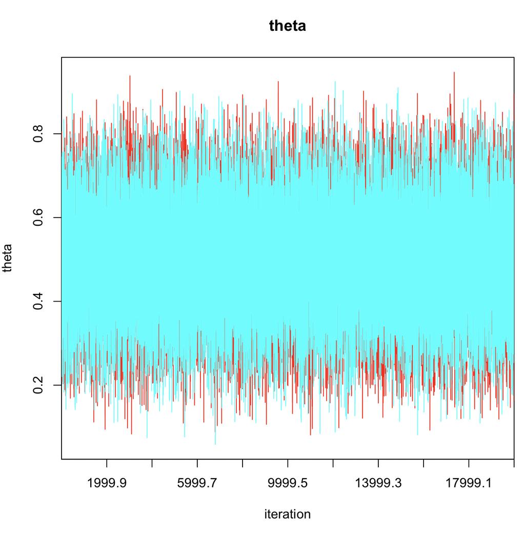
18 traceplot は R2jags の関数

19 > summary(theta) V1 Min. : st Qu.: Median : Mean : rd Qu.: Max. : chain1 の θ chain2 の θ > max(c(samples$bugsoutput$sims.array[,1,][,2], samples$bugsoutput$sims.array[,2,][1,2])) [1] > min(c(samples$bugsoutput$sims.array[,1,][,2], samples$bugsoutput$sims.array[,2,][,2])) [1] > summary(c(samples$bugsoutput$sims.array[,1,][,2], samples$bugsoutput$sims.array[,2,][,2 Min. 1st Qu. Median Mean 3rd Qu. Max

20 ベイズ統計で実践モデリング 3.2 2つの率の差第 3 章項分布を使った推論

21 違うコインでそれぞれコイントス n 1 回トス, k 1 回表が出る n 2 回トス, k 2 回表が出る表が出る率 θ 1 表が出る率 θ 2

22 δ k = ~B n =, θ = k E ~B n E, θ E 尤度 θ 1 θ 2 θ = ~Beta(1,1) θ E ~Beta(1,1) 事前分布 k 1 k 2 δ θ = θ E 率の差 n 1 n 2 確定変数 (deterministic variable) を表すノード

23 Rate_2.txt # Difference Between Two Rates model{ # Observed Counts } k1 ~ dbin(theta1,n1) k2 ~ dbin(theta2,n2) # Prior on Rates theta1 ~ dbeta(1,1) theta2 ~ dbeta(1,1) 尤度事前分布 # Difference Between Rates delta <- theta1-theta2

24 R2jags による MCMC サンプリング Rate_2_jags.R 変数のクリア # clears workspace: rm(list=ls()) Rate_2.txt と Rate_2_jags.R のあるディレクトリへの移動 # sets working directories: setwd("/users/toh/desktop/code/parameterestimation/binomial") library(r2jags) パッケージの読み込み k1 <- 5 k2 <- 7 n1 <- 10 n2 <- 10 data <- list("k1", "k2", "n1", "n2") # to be passed on to JAGS 観測変数の設定

25 θ 1 と θ 2 の初期値の設定何故 list(list()) となっているのか? ヒント :n.chains の設定 myinits <- list( list(theta1 = 0.1, theta2 = 0.9)) # parameters to be monitored: parameters <- c("delta", "theta1", "theta2") モニターするパラメータの設定 # The following command calls JAGS with specific options. # For a detailed description see the R2jags documentation. samples <- jags(data, inits=myinits, parameters, model.file ="Rate_2.txt", n.chains=1, n.iter=10000, n.burnin=1, n.thin=1, DIC=T) Jags を呼び出して θ をサンプリング

26 サンプリングされた δ( 率の差 ) を取り出してその事後分布を作成 delta <- samples$bugsoutput$sims.list$delta # Now let's plot a histogram for delta. # First, some options to make the plot look better: par(cex.main = 1.5, mar = c(5, 6, 4, 5) + 0.1, mgp = c(3.5, 1, 0), cex.lab = 1.5, font.lab = 2, cex.axis = 1.3, bty = "n", las=1) Nbreaks <- 80 y <- hist(delta, Nbreaks, plot=f) plot(c(y$breaks, max(y$breaks)), c(0,y$density,0), type="s", lwd=2, lty=1, xlim=c(-1,1), ylim=c(0,10), xlab="difference in Rates", ylab="posterior Density")

28 δ の点推定, 区間推定 # mean of delta: mean(delta) # median of delta: median(delta) # mode of delta, estimated from the "density" smoother: density(delta)$x[which(density(delta)$y==max(density(delta)$y))] # 95% credible interval for delta: quantile(delta, c(.025,.975))

29 > mean(delta) [1] 平均 > median(delta) [1] メジアン > density(delta)$x[which(density(delta)$y==max(density(delta)$y))] [1] モード > quantile(delta, c(.025,.975)) 2.5% 97.5% % 信区間

30 ベイズ統計で実践モデリング 3.3 共通の率を推論する第 3 章項分布を使った推論

31 同じコインを 2 が独にコイントス n 1 回トス, k 1 回表が出る n 2 回トス, k 2 回表が出る表が出る率 θ

32 θ k = ~B n =, θ k E ~B n E, θ 尤度 k 1 k 2 θ~beta(1,1) 事前分布 n 1 n 2

33 θ k i k H ~B n H, θ θ~beta(1,1) 尤度事前分布 n i i 独なグラフの繰り返しを閉じた形で囲んで表す for ループのような表現

34 Rate_3.txt # Inferring a Common Rate model{ # Observed Counts k1 ~ dbin(theta,n1) 尤度 k2 ~ dbin(theta,n2) # Prior on Single Rate Theta theta ~ dbeta(1,1) 事前分布 }

35 Rate_3_jags.R 変数のクリア # clears workspace: rm(list=ls()) Rate_2.txt と Rate_2_jags.R のあるディレクトリへの移動 # sets working directories: setwd("/users/toh/desktop/code/parameterestimation/binomial") library(r2jags) パッケージの読み込み k1 <- 5 k2 <- 7 n1 <- 10 n2 <- 10 data <- list("k1", "k2", "n1", "n2") # to be passed on to JAGS 観測変数の設定

36 θ の初期値の設定 myinits <- list( list(theta = 0.5)) # parameters to be monitored: parameters <- c("theta") モニターするパラメータの設定 # The following command calls JAGS with specific options. # For a detailed description see the R2jags documentation. samples <- jags(data, inits=myinits, parameters, model.file ="Rate_3.txt", n.chains=1, n.iter=1000, n.burnin=1, n.thin=1, DIC=T) Jags を呼び出して θ をサンプリング

37 samples の中から θ のサンプルを取り出す theta <- samples$bugsoutput$sims.list$theta # Now let's plot a histogram for theta. # First, some options to make the plot look better: par(cex.main = 1.5, mar = c(5, 6, 4, 5) + 0.1, mgp = c(3.5, 1, 0), cex.lab = 1.5, font.lab = 2, cex.axis = 1.3, bty = "n", las=1) Nbreaks <- 80 y <- hist(theta, Nbreaks, plot=f) plot(c(y$breaks, max(y$breaks)), c(0,y$density,0), type="s", lwd=2, lty=1, xlim=c(0,1), ylim=c(0,10), xlab="rate", ylab="posterior Density") θ の事後分布をプロット

39 > mean(theta) [1] > median(theta) [1] > density(theta)$x[which(density(theta)$y==max(density(theta)$y))] [1] > quantile(theta, c(.025,.975)) 2.5% 97.5%

40 まとめ問題からグラフィカルモデルを作るグラフィカルモデルから jags のモデルを記述する R のスクリプトを記述 (1) ワークスペースへの移動 (2) ワークスペースのクリア (3)R2jags の読み込み (4) 観測データの記述 (5) パラメータの初期値の設定 (6) モニターするパラメータの設定 (7)Jags を実し MCMC によるサンプリングを実 (8) サンプリング結果を可視化点推定区間推定

バイオインフォマティクス特論12

バイオインフォマティクス特論12 藤博幸事後予測分布パラメータの事後分布に従ってモデルがどんなデータを期待するかを予測する予測分布が観測されたデータと致するかを確認することでモデルの適切さを確認できる前回と同じ問題で事後予測をう 3-1-1. 個差を考えない場合 3-1-2. 完全な個差を考える場合 3-1-3. 構造化された個差を考える場合ベイズ統計で実践モデリング 10.1 個差を考えない場合第 10