( )
|
|
|
- みひな やすもと
- 7 years ago
- Views:
Transcription
")
1 ( )

 SDSS : d 2 r i dt 2 = Gm jr")
2 () ( ) SDSS : d 2 r i dt 2 = Gm jr ij j i rij 3
3 = Newton 3 0.1% 19
4 ( ) 3 3 (2 )

5 ,3 Sun L4 L5 Jupiter Figure-8 solution 10 Figure-8 Solution 3 (0.005% )
6 d 2 x = f(x) (1) dt2 x(0) = x 0, dx dt t=0 = v(0) = v 0 (2) 1 dx/dt = f(x) x(t +Δt) =x(t)+δtf(x(t))

7 e Nature : Laskar and Gastineau 2009 ( 0.38mm)
8 1 2
9 = /10
10 ρ R d 2 R dt = πgρr3 /R 2 = 4 πgρr (3) 3 d 2 r dt 2 = 4 3 πgm/r2 (4) M ρr 3 a(t) ρ(t) =ρ 0 /a 3, r = r 0 a (5) 2 a d 2 a dt 2 = 4 3 πρ 0/a 2 (6) 3 2 a 0 t
11 ( ) )
12 ? X X 2 Hot dark matter Cold dark matter
13 1
14 Ill-posed problem??
15 f(x, v) :6 f(x, v)dxdv dxdv f t + v f Φ f v =0, (7) Φ 2 φ = 4πGρ. (8) G ρ ρ = m dvf, (9)
16 . 1996

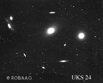
17 M82 X NASA Chandra X
18 2 2 D = D
19
20 f t = A(f(x)) (10) ( A f 2) (1) df df f 0 (x) A(f 0 (x)) = 0 f = f 0 + df df (2) : df f 0 df : df t = B(df (x)) (11) B(αdf 1 (x)+βdf 2 (x)) = αb(df 1 (x))+βb(df 2 (x)) (12) (3) df 1 df 1 df 1, df 2 df 1 + df 2
21 λ λdf = B(df ) (13) df = e λt df 0 λ f 0 f 0 df df
22 , D =1.05 (2), D =10 λ: (3), D = 100, D = 709
23 , D = 1000 gravothermal instavility V. Antnov (1961) : Hachisu & Sugimoto (1978) Hachisu et al. (1978) : Cohn (1980):
24 3 (Nature Vol 428 No , Formation of massive black holes through runaway collisions in dense young star clusters ) 1. : 2. M82 IMBH 3. : Classic View (Rees 1984) 2...
25 () ( ) 3 merger : ( ) M82 BH Matsumoto et al. ApJL 547, L25 BH 10M BH > 10 6 M
26 M82 IMBH ( ) () >> 10, << 10 6 BH M82 (K band) 700M = IMBH (intermediate-mass BH). M : BH (2) HST NICMOS/Keck NIRSPEC McCrady et al. (astro-ph/ ) IMBH ( ) IMBH IMBH How IMBHs were formed? ()
27 McCrady et al (astro-ph/ ) Cluster #11 (MGG-11) σ r =11.4 ± 0.8km/s half-light radius 1.2 ± 0.17pc IMBH ( ) 3. IMBH ( ) kinetic mass 3.5 ± M Age 10Myrs. M/L ( ) (< 10 Myrs) King model with W 0 = 7-12 Salpeter IMF (as suggested by McCrady et al) Star-by-star simulation for MGG-11 (MGG-9 is scaled) W 0 8 (MGG-11 ) MGG-9 ( )
 2MASS Chandra M82-X1 MGG11 0.")
28 ( ) BH M ( ) IMBH IMBH IMBH / M82 IMBH ( ) (BH2003 talk) 2MASS Chandra M82-X1 MGG Radiation recoil


29 IMBH SMBH Merger SMBH Growth timescale would be too large 3. SMBH IMBH? ( ) Ebisuzaki et al ApJ 562, 19L 1) 2).... 3) 4) IMBH 3. IMBH 4. IMBH IMBH Katz and Gunn 1992 : Cray YMP : 1000

30 Saitoh et al animation GRAPE-5 1 (!) 1 : 1 : 1 : 4-5 :

 1 2 SPH Cray XT4 ASURA 10pc")
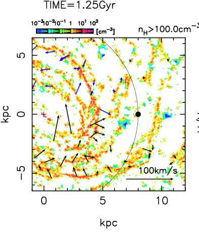
31 Saitoh et al Star formation with SPH Large scale structure formation with AMR animation (Baba et al 2009) 1 2 SPH Cray XT4 ASURA 10pc ( 500pc) 10K ( 10 4 K) 3000M ( 10 5 M )


32 2006: Xu et al, Science 311, 54 Nov 2008: Burst of results from VLBA Several data from VERA (Compiled by Dr. Asaki)

33 ( 30km/s)
 animation a1 animation a2 animation")

34 ( ) ( ) + (Fujii et al. 2010) animation a1 animation a2 animation b1 Stable against radial mode (a1, a2) Spiral arms form They seem to be maintained for very long time
35
36 148Gflops Gflops 10 (GRAVITY PIPE, GRAPE) GRAPE Host Computer Time integration etc. GRAPE Interaction calculation : :


37 GRAPE 1988 GRAPE GRAPE
38 GRAPE GRAPE = GRAPE: 1/100 GRAPE-6 ( ()) μm μm nm nm 10 GRAPE-DR :


39 GRAPE-DR R i = j f(x i,y j ) (M) 2 y j PEID BBID A x + ALU B T 32W 256W 256 (K M ) W MHz Gflops PCIe 20

40 GRAPE-DR GRAPE-DR : 128-, 128- (105Tflops peak) : Intel Core i7+x GB : x4 DDR LU ( 1A: CPU 2 ) 430Gflops(1 ) 670Gflops(2 ) 1 CPU 11 GDR 4 chips GDR 1 chips GRAPE-6 HD5870 Performance for small N much better than GPU (for treecode, the multiwalk method greatly improves GPU performance, though)

41 Little Green 500, June 2010 (nm) (GF/W) GRAPE-DR GRAPE Tesla C Xeon #2: IBM PowerXCell, #9: NVIDIA Fermi GRAPE-DR 10 GRAPE-6 GRAPE-6 10 : 30 GRAPE-DR FPGA ASIC
42 2 : % A Green /24
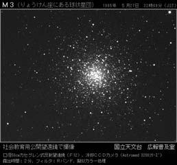
 1. : 1.5 2. ( ): 2.5 3. : 1 ( ) / minimum solar nebula model ( ) http://antwrp.gsfc.nasa.gov/apod/ap950917.html ( ) http://www-astro.physics.ox.ac.uk/~wjs/apm_grey.gif ( ) SDSS : d 2 r i dt 2 ÿ j i
EGunGPU
 Super Computing in Accelerator simulations - Electron Gun simulation using GPGPU - K. Ohmi, KEK-Accel Accelerator Physics seminar 2009.11.19 Super computers in KEK HITACHI SR11000 POWER5 16 24GB 16 134GFlops,
SFN
 THE STAR FORMATION NEWSLETTER No.291-14 March 2017 2017/04/28 16-20 16. X-Shooter spectroscopy of young stellar objects in Lupus. Atmospheric parameters, membership and activity diagnostics 17. The evolution
23 Fig. 2: hwmodulev2 3. Reconfigurable HPC 3.1 hw/sw hw/sw hw/sw FPGA PC FPGA PC FPGA HPC FPGA FPGA hw/sw hw/sw hw- Module FPGA hwmodule hw/sw FPGA h
 23 FPGA CUDA Performance Comparison of FPGA Array with CUDA on Poisson Equation ([email protected]), ([email protected]), ([email protected]), ([email protected]),
1 (Berry,1975) 2-6 p (S πr 2 )p πr 2 p 2πRγ p p = 2γ R (2.5).1-1 : : : : ( ).2 α, β α, β () X S = X X α X β (.1) 1 2
 2-6 p (S πr 2 )p πr 2 p 2πRγ p p = 2γ R (2.5).1-1 : : : : ( ).2 α, β α, β () X S = X X α X β (.1) 1 2") 2005 9/8-11 2 2.2 ( 2-5) γ ( ) γ cos θ 2πr πρhr 2 g h = 2γ cos θ ρgr (2.1) γ = ρgrh (2.2) 2 cos θ θ cos θ = 1 (2.2) γ = 1 ρgrh (2.) 2 2. p p ρgh p ( ) p p = p ρgh (2.) h p p = 2γ r 1 1 (Berry,1975) 2-6
2005 9/8-11 2 2.2 ( 2-5) γ ( ) γ cos θ 2πr πρhr 2 g h = 2γ cos θ ρgr (2.1) γ = ρgrh (2.2) 2 cos θ θ cos θ = 1 (2.2) γ = 1 ρgrh (2.) 2 2. p p ρgh p ( ) p p = p ρgh (2.) h p p = 2γ r 1 1 (Berry,1975) 2-6
sec13.dvi
 13 13.1 O r F R = m d 2 r dt 2 m r m = F = m r M M d2 R dt 2 = m d 2 r dt 2 = F = F (13.1) F O L = r p = m r ṙ dl dt = m ṙ ṙ + m r r = r (m r ) = r F N. (13.2) N N = R F 13.2 O ˆn ω L O r u u = ω r 1 1:
Note.tex 2008/09/19( )
") 1 20 9 19 2 1 5 1.1........................ 5 1.2............................. 8 2 9 2.1............................. 9 2.2.............................. 10 3 13 3.1.............................. 13 3.2..................................
1 20 9 19 2 1 5 1.1........................ 5 1.2............................. 8 2 9 2.1............................. 9 2.2.............................. 10 3 13 3.1.............................. 13 3.2..................................
 http://www.ns.kogakuin.ac.jp/~ft13389/lecture/physics1a2b/ pdf I 1 1 1.1 ( ) 1. 30 m µm 2. 20 cm km 3. 10 m 2 cm 2 4. 5 cm 3 km 3 5. 1 6. 1 7. 1 1.2 ( ) 1. 1 m + 10 cm 2. 1 hr + 6400 sec 3. 3.0 10 5 kg
1 (1) () (3) I 0 3 I I d θ = L () dt θ L L θ I d θ = L = κθ (3) dt κ T I T = π κ (4) T I κ κ κ L l a θ L r δr δl L θ ϕ ϕ = rθ (5) l
 () (3) I 0 3 I I d θ = L () dt θ L L θ I d θ = L = κθ (3) dt κ T I T = π κ (4) T I κ κ κ L l a θ L r δr δl L θ ϕ ϕ = rθ (5) l") 1 1 ϕ ϕ ϕ S F F = ϕ (1) S 1: F 1 1 (1) () (3) I 0 3 I I d θ = L () dt θ L L θ I d θ = L = κθ (3) dt κ T I T = π κ (4) T I κ κ κ L l a θ L r δr δl L θ ϕ ϕ = rθ (5) l : l r δr θ πrδr δf (1) (5) δf = ϕ πrδr
1 1 ϕ ϕ ϕ S F F = ϕ (1) S 1: F 1 1 (1) () (3) I 0 3 I I d θ = L () dt θ L L θ I d θ = L = κθ (3) dt κ T I T = π κ (4) T I κ κ κ L l a θ L r δr δl L θ ϕ ϕ = rθ (5) l : l r δr θ πrδr δf (1) (5) δf = ϕ πrδr

PowerPoint Presentation
 2010 KEK (Japan) (Japan) (Japan) Cheoun, Myun -ki Soongsil (Korea) Ryu,, Chung-Yoe Soongsil (Korea) 1. S.Reddy, M.Prakash and J.M. Lattimer, P.R.D58 #013009 (1998) Magnetar : ~ 10 15 G ~ 10 17 19 G (?)

研修コーナー
 l l l l l l l l l l l α α β l µ l l l l l l l l l l l l l l l l l l l l l l l l l l l l l l l l l l l l l l l l l l l l l l l l l l l l l l l l l l l l l l l l l l l l l l l l l l l l l l
(1.2) T D = 0 T = D = 30 kn 1.2 (1.4) 2F W = 0 F = W/2 = 300 kn/2 = 150 kn 1.3 (1.9) R = W 1 + W 2 = = 1100 N. (1.9) W 2 b W 1 a = 0
 T D = 0 T = D = 30 kn 1.2 (1.4) 2F W = 0 F = W/2 = 300 kn/2 = 150 kn 1.3 (1.9) R = W 1 + W 2 = = 1100 N. (1.9) W 2 b W 1 a = 0") 1 1 1.1 1.) T D = T = D = kn 1. 1.4) F W = F = W/ = kn/ = 15 kn 1. 1.9) R = W 1 + W = 6 + 5 = 11 N. 1.9) W b W 1 a = a = W /W 1 )b = 5/6) = 5 cm 1.4 AB AC P 1, P x, y x, y y x 1.4.) P sin 6 + P 1 sin 45
1 1 1.1 1.) T D = T = D = kn 1. 1.4) F W = F = W/ = kn/ = 15 kn 1. 1.9) R = W 1 + W = 6 + 5 = 11 N. 1.9) W b W 1 a = a = W /W 1 )b = 5/6) = 5 cm 1.4 AB AC P 1, P x, y x, y y x 1.4.) P sin 6 + P 1 sin 45
")
64 3 g=9.85 m/s 2 g=9.791 m/s 2 36, km ( ) 1 () 2 () m/s : : a) b) kg/m kg/m k
 1 () 2 () m/s : : a) b) kg/m kg/m k") 63 3 Section 3.1 g 3.1 3.1: : 64 3 g=9.85 m/s 2 g=9.791 m/s 2 36, km ( ) 1 () 2 () 3 9.8 m/s 2 3.2 3.2: : a) b) 5 15 4 1 1. 1 3 14. 1 3 kg/m 3 2 3.3 1 3 5.8 1 3 kg/m 3 3 2.65 1 3 kg/m 3 4 6 m 3.1. 65 5
63 3 Section 3.1 g 3.1 3.1: : 64 3 g=9.85 m/s 2 g=9.791 m/s 2 36, km ( ) 1 () 2 () 3 9.8 m/s 2 3.2 3.2: : a) b) 5 15 4 1 1. 1 3 14. 1 3 kg/m 3 2 3.3 1 3 5.8 1 3 kg/m 3 3 2.65 1 3 kg/m 3 4 6 m 3.1. 65 5
医系の統計入門第 2 版 サンプルページ この本の定価 判型などは, 以下の URL からご覧いただけます. このサンプルページの内容は, 第 2 版 1 刷発行時のものです.
 医系の統計入門第 2 版 サンプルページ この本の定価 判型などは, 以下の URL からご覧いただけます. http://www.morikita.co.jp/books/mid/009192 このサンプルページの内容は, 第 2 版 1 刷発行時のものです. i 2 t 1. 2. 3 2 3. 6 4. 7 5. n 2 ν 6. 2 7. 2003 ii 2 2013 10 iii 1987
2 2 1?? 2 1 1, 2 1, 2 1, 2, 3,... 1, 2 1, 3? , 2 2, 3? k, l m, n k, l m, n kn > ml...? 2 m, n n m
 2009 IA I 22, 23, 24, 25, 26, 27 4 21 1 1 2 1! 4, 5 1? 50 1 2 1 1 2 1 4 2 2 2 1?? 2 1 1, 2 1, 2 1, 2, 3,... 1, 2 1, 3? 2 1 3 1 2 1 1, 2 2, 3? 2 1 3 2 3 2 k, l m, n k, l m, n kn > ml...? 2 m, n n m 3 2
2 7 V 7 {fx fx 3 } 8 P 3 {fx fx 3 } 9 V 9 {fx fx f x 2fx } V {fx fx f x 2fx + } V {{a n } {a n } a n+2 a n+ + a n n } 2 V 2 {{a n } {a n } a n+2 a n+
 R 3 R n C n V??,?? k, l K x, y, z K n, i x + y + z x + y + z iv x V, x + x o x V v kx + y kx + ky vi k + lx kx + lx vii klx klx viii x x ii x + y y + x, V iii o K n, x K n, x + o x iv x K n, x + x o x
Contents 1 Jeans (
 Contents 1 Jeans 2 1.1....................................... 2 1.2................................. 2 1.3............................... 3 2 3 2.1 ( )................................ 4 2.2 WKB........................
非線形長波モデルと流体粒子法による津波シミュレータの開発 I_ m ρ v p h g a b a 2h b r ab a b Fang W r ab h 5 Wendland 1995 q= r ab /h a d W r ab h
 土木学会論文集 B2( 海岸工学 ) Vol. 70, No. 2, 2014, I_016-I_020 非線形長波モデルと流体粒子法による津波シミュレータの開発 Development of a Tsunami Simulator Integrating the Smoothed-Particle Hydrodynamics Method and the Nonlinear Shallow Water
2000年度『数学展望 I』講義録
 2000 I I IV I II 2000 I I IV I-IV. i ii 3.10 (http://www.math.nagoya-u.ac.jp/ kanai/) 2000 A....1 B....4 C....10 D....13 E....17 Brouwer A....21 B....26 C....33 D....39 E. Sperner...45 F....48 A....53
all.dvi
 72 9 Hooke,,,. Hooke. 9.1 Hooke 1 Hooke. 1, 1 Hooke. σ, ε, Young. σ ε (9.1), Young. τ γ G τ Gγ (9.2) X 1, X 2. Poisson, Poisson ν. ν ε 22 (9.) ε 11 F F X 2 X 1 9.1: Poisson 9.1. Hooke 7 Young Poisson G
爆発的星形成? AGN関係を 生み出す物理機構の観測的示唆
 Umemura, Fukue & Mineshige 1997, 1998 Ohsuga et al. 1998 R ring ~100pc dv r = v 2 ϕ dt r 1 dp ρ dr dφ 1 r d(rv ϕ ) dt = 3χE 2c typical timescale dr + χ c F r 3 2 Myr r R ring V ring 3χE 2c v ϕ Umemura,
 20 4 20 i 1 1 1.1............................ 1 1.2............................ 4 2 11 2.1................... 11 2.2......................... 11 2.3....................... 19 3 25 3.1.............................
 21 2 26 i 1 1 1.1............................ 1 1.2............................ 3 2 9 2.1................... 9 2.2.......... 9 2.3................... 11 2.4....................... 12 3 15 3.1..........
untitled
 SPring-8 RFgun JASRI/SPring-8 6..7 Contents.. 3.. 5. 6. 7. 8. . 3 cavity γ E A = er 3 πε γ vb r B = v E c r c A B A ( ) F = e E + v B A A A A B dp e( v B+ E) = = m d dt dt ( γ v) dv e ( ) dt v B E v E
TOP URL 1
 TOP URL http://amonphys.web.fc.com/ 3.............................. 3.............................. 4.3 4................... 5.4........................ 6.5........................ 8.6...........................7
W u = u(x, t) u tt = a 2 u xx, a > 0 (1) D := {(x, t) : 0 x l, t 0} u (0, t) = 0, u (l, t) = 0, t 0 (2)
 u tt = a 2 u xx, a > 0 (1) D := {(x, t) : 0 x l, t 0} u (0, t) = 0, u (l, t) = 0, t 0 (2)") 3 215 4 27 1 1 u u(x, t) u tt a 2 u xx, a > (1) D : {(x, t) : x, t } u (, t), u (, t), t (2) u(x, ) f(x), u(x, ) t 2, x (3) u(x, t) X(x)T (t) u (1) 1 T (t) a 2 T (t) X (x) X(x) α (2) T (t) αa 2 T (t) (4)
3 215 4 27 1 1 u u(x, t) u tt a 2 u xx, a > (1) D : {(x, t) : x, t } u (, t), u (, t), t (2) u(x, ) f(x), u(x, ) t 2, x (3) u(x, t) X(x)T (t) u (1) 1 T (t) a 2 T (t) X (x) X(x) α (2) T (t) αa 2 T (t) (4)
42 3 u = (37) MeV/c 2 (3.4) [1] u amu m p m n [1] m H [2] m p = (4) MeV/c 2 = (13) u m n = (4) MeV/c 2 =
![42 3 u = (37) MeV/c 2 (3.4) [1] u amu m p m n [1] m H [2] m p = (4) MeV/c 2 = (13) u m n = (4) MeV/c 2 =](/thumbs/73/68712188.jpg "42 3 u = (37) MeV/c 2 (3.4) [1] u amu m p m n [1] m H [2] m p = (4) MeV/c 2 = (13) u m n = (4) MeV/c 2 =") 3 3.1 3.1.1 kg m s J = kg m 2 s 2 MeV MeV [1] 1MeV=1 6 ev = 1.62 176 462 (63) 1 13 J (3.1) [1] 1MeV/c 2 =1.782 661 731 (7) 1 3 kg (3.2) c =1 MeV (atomic mass unit) 12 C u = 1 12 M(12 C) (3.3) 41 42 3 u
3 3.1 3.1.1 kg m s J = kg m 2 s 2 MeV MeV [1] 1MeV=1 6 ev = 1.62 176 462 (63) 1 13 J (3.1) [1] 1MeV/c 2 =1.782 661 731 (7) 1 3 kg (3.2) c =1 MeV (atomic mass unit) 12 C u = 1 12 M(12 C) (3.3) 41 42 3 u
2011de.dvi
 211 ( 4 2 1. 3 1.1............................... 3 1.2 1- -......................... 13 1.3 2-1 -................... 19 1.4 3- -......................... 29 2. 37 2.1................................ 37
No.004 [1] J. ( ) ( ) (1968) [2] Morse (1997) [3] (1988) 1
![No.004 [1] J. ( ) ( ) (1968) [2] Morse (1997) [3] (1988) 1](/thumbs/94/119152523.jpg "No.004 [1] J. ( ) ( ) (1968) [2] Morse (1997) [3] (1988) 1") No.004 [1] J. ( ) ( ) (1968) [2] Morse (1997) [3] (1988) 1 1 (1) 1.1 X Y f, g : X Y { F (x, 0) = f(x) F (x, 1) = g(x) F : X I Y f g f g F f g 1.2 X Y X Y gf id X, fg id Y f : X Y, g : Y X X Y X Y (2) 1.3
No.004 [1] J. ( ) ( ) (1968) [2] Morse (1997) [3] (1988) 1 1 (1) 1.1 X Y f, g : X Y { F (x, 0) = f(x) F (x, 1) = g(x) F : X I Y f g f g F f g 1.2 X Y X Y gf id X, fg id Y f : X Y, g : Y X X Y X Y (2) 1.3
 B 1 B.1.......................... 1 B.1.1................. 1 B.1.2................. 2 B.2........................... 5 B.2.1.......................... 5 B.2.2.................. 6 B.2.3..................
1: 3.3 1/8000 1/ m m/s v = 2kT/m = 2RT/M k R 8.31 J/(K mole) M 18 g 1 5 a v t πa 2 vt kg (
 M 18 g 1 5 a v t πa 2 vt kg (") 1905 1 1.1 0.05 mm 1 µm 2 1 1 2004 21 2004 7 21 2005 web 2 [1, 2] 1 1: 3.3 1/8000 1/30 3 10 10 m 3 500 m/s 4 1 10 19 5 6 7 1.2 3 4 v = 2kT/m = 2RT/M k R 8.31 J/(K mole) M 18 g 1 5 a v t πa 2 vt 6 6 10
1905 1 1.1 0.05 mm 1 µm 2 1 1 2004 21 2004 7 21 2005 web 2 [1, 2] 1 1: 3.3 1/8000 1/30 3 10 10 m 3 500 m/s 4 1 10 19 5 6 7 1.2 3 4 v = 2kT/m = 2RT/M k R 8.31 J/(K mole) M 18 g 1 5 a v t πa 2 vt 6 6 10
A Feasibility Study of Direct-Mapping-Type Parallel Processing Method to Solve Linear Equations in Load Flow Calculations Hiroaki Inayoshi, Non-member
 A Feasibility Study of Direct-Mapping-Type Parallel Processing Method to Solve Linear Equations in Load Flow Calculations Hiroaki Inayoshi, Non-member (University of Tsukuba), Yasuharu Ohsawa, Member (Kobe
GPGPU
 GPGPU 2013 1008 2015 1 23 Abstract In recent years, with the advance of microscope technology, the alive cells have been able to observe. On the other hand, from the standpoint of image processing, the
Gmech08.dvi
 145 13 13.1 13.1.1 0 m mg S 13.1 F 13.1 F /m S F F 13.1 F mg S F F mg 13.1: m d2 r 2 = F + F = 0 (13.1) 146 13 F = F (13.2) S S S S S P r S P r r = r 0 + r (13.3) r 0 S S m d2 r 2 = F (13.4) (13.3) d 2
スライド 1
 Matsuura Laboratory SiC SiC 13 2004 10 21 22 H-SiC ( C-SiC HOY Matsuura Laboratory n E C E D ( E F E T Matsuura Laboratory Matsuura Laboratory DLTS Osaka Electro-Communication University Unoped n 3C-SiC
S I. dy fx x fx y fx + C 3 C vt dy fx 4 x, y dy yt gt + Ct + C dt v e kt xt v e kt + C k x v k + C C xt v k 3 r r + dr e kt S Sr πr dt d v } dt k e kt
 S I. x yx y y, y,. F x, y, y, y,, y n http://ayapin.film.s.dendai.ac.jp/~matuda n /TeX/lecture.html PDF PS yx.................................... 3.3.................... 9.4................5..............
³ÎΨÏÀ
 2017 12 12 Makoto Nakashima 2017 12 12 1 / 22 2.1. C, D π- C, D. A 1, A 2 C A 1 A 2 C A 3, A 4 D A 1 A 2 D Makoto Nakashima 2017 12 12 2 / 22 . (,, L p - ). Makoto Nakashima 2017 12 12 3 / 22 . (,, L p
inflation.key
 2 2 G M 0 0-5 ϕ / M G 0 L SUGRA = 1 2 er + eg ij Dµ φ i Dµ φ j 1 2 eg2 D (a) D +ieg ij χ j σ µ Dµ χ i + eϵ µνρσ ψ µ σ ν Dρ ψ σ 1 4 ef (ab) R F (a) [ ] + i 2 e λ (a) σ µ Dµ λ (a) + λ (a) σ µ Dµ λ (a) 1
nsg02-13/ky045059301600033210
 φ φ φ φ κ κ α α μ μ α α μ χ et al Neurosci. Res. Trpv J Physiol μ μ α α α β in vivo β β β β β β β β in vitro β γ μ δ μδ δ δ α θ α θ α In Biomechanics at Micro- and Nanoscale Levels, Volume I W W v W
 215 11 13 1 2 1.1....................... 2 1.2.................... 2 1.3..................... 2 1.4...................... 3 1.5............... 3 1.6........................... 4 1.7.................. 4
 IA [email protected] Last updated: January,......................................................................................................................................................................................
JFE.dvi
 ,, Department of Civil Engineering, Chuo University Kasuga 1-13-27, Bunkyo-ku, Tokyo 112 8551, JAPAN E-mail : [email protected] E-mail : [email protected] SATO KOGYO CO., LTD. 12-20, Nihonbashi-Honcho
DVIOUT
 A. A. A-- [ ] f(x) x = f 00 (x) f 0 () =0 f 00 () > 0= f(x) x = f 00 () < 0= f(x) x = A--2 [ ] f(x) D f 00 (x) > 0= y = f(x) f 00 (x) < 0= y = f(x) P (, f()) f 00 () =0 A--3 [ ] y = f(x) [, b] x = f (y)
I-2 (100 ) (1) y(x) y dy dx y d2 y dx 2 (a) y + 2y 3y = 9e 2x (b) x 2 y 6y = 5x 4 (2) Bernoulli B n (n = 0, 1, 2,...) x e x 1 = n=0 B 0 B 1 B 2 (3) co
 (1) y(x) y dy dx y d2 y dx 2 (a) y + 2y 3y = 9e 2x (b) x 2 y 6y = 5x 4 (2) Bernoulli B n (n = 0, 1, 2,...) x e x 1 = n=0 B 0 B 1 B 2 (3) co") 16 I ( ) (1) I-1 I-2 I-3 (2) I-1 ( ) (100 ) 2l x x = 0 y t y(x, t) y(±l, t) = 0 m T g y(x, t) l y(x, t) c = 2 y(x, t) c 2 2 y(x, t) = g (A) t 2 x 2 T/m (1) y 0 (x) y 0 (x) = g c 2 (l2 x 2 ) (B) (2) (1)
16 I ( ) (1) I-1 I-2 I-3 (2) I-1 ( ) (100 ) 2l x x = 0 y t y(x, t) y(±l, t) = 0 m T g y(x, t) l y(x, t) c = 2 y(x, t) c 2 2 y(x, t) = g (A) t 2 x 2 T/m (1) y 0 (x) y 0 (x) = g c 2 (l2 x 2 ) (B) (2) (1)
p = mv p x > h/4π λ = h p m v Ψ 2 Ψ
 II p = mv p x > h/4π λ = h p m v Ψ 2 Ψ Ψ Ψ 2 0 x P'(x) m d 2 x = mω 2 x = kx = F(x) dt 2 x = cos(ωt + φ) mω 2 = k ω = m k v = dx = -ωsin(ωt + φ) dt = d 2 x dt 2 0 y v θ P(x,y) θ = ωt + φ ν = ω [Hz] 2π
2 1 κ c(t) = (x(t), y(t)) ( ) det(c (t), c x (t)) = det (t) x (t) y (t) y = x (t)y (t) x (t)y (t), (t) c (t) = (x (t)) 2 + (y (t)) 2. c (t) =
 = (x(t), y(t)) ( ) det(c (t), c x (t)) = det (t) x (t) y (t) y = x (t)y (t) x (t)y (t), (t) c (t) = (x (t)) 2 + (y (t)) 2. c (t) =") 1 1 1.1 I R 1.1.1 c : I R 2 (i) c C (ii) t I c (t) (0, 0) c (t) c(i) c c(t) 1.1.2 (1) (2) (3) (1) r > 0 c : R R 2 : t (r cos t, r sin t) (2) C f : I R c : I R 2 : t (t, f(t)) (3) y = x c : R R 2 : t (t,
1 1 1.1 I R 1.1.1 c : I R 2 (i) c C (ii) t I c (t) (0, 0) c (t) c(i) c c(t) 1.1.2 (1) (2) (3) (1) r > 0 c : R R 2 : t (r cos t, r sin t) (2) C f : I R c : I R 2 : t (t, f(t)) (3) y = x c : R R 2 : t (t,
x A Aω ẋ ẋ 2 + ω 2 x 2 = ω 2 A 2. (ẋ, ωx) ζ ẋ + iωx ζ ζ dζ = ẍ + iωẋ = ẍ + iω(ζ iωx) dt dζ dt iωζ = ẍ + ω2 x (2.1) ζ ζ = Aωe iωt = Aω cos ωt + iaω sin
 ζ ẋ + iωx ζ ζ dζ = ẍ + iωẋ = ẍ + iω(ζ iωx) dt dζ dt iωζ = ẍ + ω2 x (2.1) ζ ζ = Aωe iωt = Aω cos ωt + iaω sin") 2 2.1 F (t) 2.1.1 mẍ + kx = F (t). m ẍ + ω 2 x = F (t)/m ω = k/m. 1 : (ẋ, x) x = A sin ωt, ẋ = Aω cos ωt 1 2-1 x A Aω ẋ ẋ 2 + ω 2 x 2 = ω 2 A 2. (ẋ, ωx) ζ ẋ + iωx ζ ζ dζ = ẍ + iωẋ = ẍ + iω(ζ iωx) dt dζ
2 2.1 F (t) 2.1.1 mẍ + kx = F (t). m ẍ + ω 2 x = F (t)/m ω = k/m. 1 : (ẋ, x) x = A sin ωt, ẋ = Aω cos ωt 1 2-1 x A Aω ẋ ẋ 2 + ω 2 x 2 = ω 2 A 2. (ẋ, ωx) ζ ẋ + iωx ζ ζ dζ = ẍ + iωẋ = ẍ + iω(ζ iωx) dt dζ
1 a b cc b * 1 Helioseismology * * r/r r/r a 1.3 FTD 9 11 Ω B ϕ α B p FTD 2 b Ω * 1 r, θ, ϕ ϕ * 2 *
 448 8542 1 e-mail: [email protected] 1. 400 400 1.1 10 1 1 5 1 11 2 3 4 656 2015 10 1 a b cc b 22 5 1.2 * 1 Helioseismology * 2 6 8 * 3 1 0.7 r/r 1.0 2 r/r 0.7 3 4 2a 1.3 FTD 9 11 Ω B ϕ α B
II ( ) (7/31) II ( [ (3.4)] Navier Stokes [ (6/29)] Navier Stokes 3 [ (6/19)] Re
![II ( ) (7/31) II ( [ (3.4)] Navier Stokes [ (6/29)] Navier Stokes 3 [ (6/19)] Re](/thumbs/94/118770263.jpg "II ( ) (7/31) II ( [ (3.4)] Navier Stokes [ (6/29)] Navier Stokes 3 [ (6/19)] Re") II 29 7 29-7-27 ( ) (7/31) II (http://www.damp.tottori-u.ac.jp/~ooshida/edu/fluid/) [ (3.4)] Navier Stokes [ (6/29)] Navier Stokes 3 [ (6/19)] Reynolds [ (4.6), (45.8)] [ p.186] Navier Stokes I Euler Navier
II 29 7 29-7-27 ( ) (7/31) II (http://www.damp.tottori-u.ac.jp/~ooshida/edu/fluid/) [ (3.4)] Navier Stokes [ (6/29)] Navier Stokes 3 [ (6/19)] Reynolds [ (4.6), (45.8)] [ p.186] Navier Stokes I Euler Navier
Sample function Re random process Flutter, Galloping, etc. ensemble (mean value) N 1 µ = lim xk( t1) N k = 1 N autocorrelation function N 1 R( t1, t1
 N 1 µ = lim xk( t1) N k = 1 N autocorrelation function N 1 R( t1, t1") Sample function Re random process Flutter, Galloping, etc. ensemble (mean value) µ = lim xk( k = autocorrelation function R( t, t + τ) = lim ( ) ( + τ) xk t xk t k = V p o o R p o, o V S M R realization
Sample function Re random process Flutter, Galloping, etc. ensemble (mean value) µ = lim xk( k = autocorrelation function R( t, t + τ) = lim ( ) ( + τ) xk t xk t k = V p o o R p o, o V S M R realization
BH BH BH BH Typeset by FoilTEX 2
 GR BH BH 2015.10.10 BH at 2015.09.07 NICT 2015.05.26 Typeset by FoilTEX 1 BH BH BH BH Typeset by FoilTEX 2 1. BH 1.1 1 Typeset by FoilTEX 3 1.2 2 A B A B t = 0 A: m a [kg] B: m b [kg] t = t f star free
. ev=,604k m 3 Debye ɛ 0 kt e λ D = n e n e Ze 4 ln Λ ν ei = 5.6π / ɛ 0 m/ e kt e /3 ν ei v e H + +e H ev Saha x x = 3/ πme kt g i g e n
 003...............................3 Debye................. 3.4................ 3 3 3 3. Larmor Cyclotron... 3 3................ 4 3.3.......... 4 3.3............ 4 3.3...... 4 3.3.3............ 5 3.4.........
all.dvi
 38 5 Cauchy.,,,,., σ.,, 3,,. 5.1 Cauchy (a) (b) (a) (b) 5.1: 5.1. Cauchy 39 F Q Newton F F F Q F Q 5.2: n n ds df n ( 5.1). df n n df(n) df n, t n. t n = df n (5.1) ds 40 5 Cauchy t l n mds df n 5.3: t
28 Horizontal angle correction using straight line detection in an equirectangular image
 28 Horizontal angle correction using straight line detection in an equirectangular image 1170283 2017 3 1 2 i Abstract Horizontal angle correction using straight line detection in an equirectangular image
数値計算:有限要素法
 ( ) 1 / 61 1 2 3 4 ( ) 2 / 61 ( ) 3 / 61 P(0) P(x) u(x) P(L) f P(0) P(x) P(L) ( ) 4 / 61 L P(x) E(x) A(x) x P(x) P(x) u(x) P(x) u(x) (0 x L) ( ) 5 / 61 u(x) 0 L x ( ) 6 / 61 P(0) P(L) f d dx ( EA du dx
V(x) m e V 0 cos x π x π V(x) = x < π, x > π V 0 (i) x = 0 (V(x) V 0 (1 x 2 /2)) n n d 2 f dξ 2ξ d f 2 dξ + 2n f = 0 H n (ξ) (ii) H
 m e V 0 cos x π x π V(x) = x < π, x > π V 0 (i) x = 0 (V(x) V 0 (1 x 2 /2)) n n d 2 f dξ 2ξ d f 2 dξ + 2n f = 0 H n (ξ) (ii) H") 199 1 1 199 1 1. Vx) m e V cos x π x π Vx) = x < π, x > π V i) x = Vx) V 1 x /)) n n d f dξ ξ d f dξ + n f = H n ξ) ii) H n ξ) = 1) n expξ ) dn dξ n exp ξ )) H n ξ)h m ξ) exp ξ )dξ = π n n!δ n,m x = Vx)
199 1 1 199 1 1. Vx) m e V cos x π x π Vx) = x < π, x > π V i) x = Vx) V 1 x /)) n n d f dξ ξ d f dξ + n f = H n ξ) ii) H n ξ) = 1) n expξ ) dn dξ n exp ξ )) H n ξ)h m ξ) exp ξ )dξ = π n n!δ n,m x = Vx)
9 2 1 f(x, y) = xy sin x cos y x y cos y y x sin x d (x, y) = y cos y (x sin x) = y cos y(sin x + x cos x) x dx d (x, y) = x sin x (y cos y) = x sin x
 = xy sin x cos y x y cos y y x sin x d (x, y) = y cos y (x sin x) = y cos y(sin x + x cos x) x dx d (x, y) = x sin x (y cos y) = x sin x") 2009 9 6 16 7 1 7.1 1 1 1 9 2 1 f(x, y) = xy sin x cos y x y cos y y x sin x d (x, y) = y cos y (x sin x) = y cos y(sin x + x cos x) x dx d (x, y) = x sin x (y cos y) = x sin x(cos y y sin y) y dy 1 sin
2009 9 6 16 7 1 7.1 1 1 1 9 2 1 f(x, y) = xy sin x cos y x y cos y y x sin x d (x, y) = y cos y (x sin x) = y cos y(sin x + x cos x) x dx d (x, y) = x sin x (y cos y) = x sin x(cos y y sin y) y dy 1 sin
H.Haken Synergetics 2nd (1978)
") 27 3 27 ) Ising Landau Synergetics Fokker-Planck F-P Landau F-P Gizburg-Landau G-L G-L Bénard/ Hopfield H.Haken Synergetics 2nd (1978) (1) Ising m T T C 1: m h Hamiltonian H = J ij S i S j h i S
27 3 27 ) Ising Landau Synergetics Fokker-Planck F-P Landau F-P Gizburg-Landau G-L G-L Bénard/ Hopfield H.Haken Synergetics 2nd (1978) (1) Ising m T T C 1: m h Hamiltonian H = J ij S i S j h i S
LLG-R8.Nisus.pdf
 d M d t = γ M H + α M d M d t M γ [ 1/ ( Oe sec) ] α γ γ = gµ B h g g µ B h / π γ g = γ = 1.76 10 [ 7 1/ ( Oe sec) ] α α = λ γ λ λ λ α γ α α H α = γ H ω ω H α α H K K H K / M 1 1 > 0 α 1 M > 0 γ α γ =
( ) sin 1 x, cos 1 x, tan 1 x sin x, cos x, tan x, arcsin x, arccos x, arctan x. π 2 sin 1 x π 2, 0 cos 1 x π, π 2 < tan 1 x < π 2 1 (1) (
 sin 1 x, cos 1 x, tan 1 x sin x, cos x, tan x, arcsin x, arccos x, arctan x. π 2 sin 1 x π 2, 0 cos 1 x π, π 2 < tan 1 x < π 2 1 (1) (") 6 20 ( ) sin, cos, tan sin, cos, tan, arcsin, arccos, arctan. π 2 sin π 2, 0 cos π, π 2 < tan < π 2 () ( 2 2 lim 2 ( 2 ) ) 2 = 3 sin (2) lim 5 0 = 2 2 0 0 2 2 3 3 4 5 5 2 5 6 3 5 7 4 5 8 4 9 3 4 a 3 b
6 20 ( ) sin, cos, tan sin, cos, tan, arcsin, arccos, arctan. π 2 sin π 2, 0 cos π, π 2 < tan < π 2 () ( 2 2 lim 2 ( 2 ) ) 2 = 3 sin (2) lim 5 0 = 2 2 0 0 2 2 3 3 4 5 5 2 5 6 3 5 7 4 5 8 4 9 3 4 a 3 b
t χ 2 F Q t χ 2 F 1 2 µ, σ 2 N(µ, σ 2 ) f(x µ, σ 2 ) = 1 ( exp (x ) µ)2 2πσ 2 2σ 2 0, N(0, 1) (100 α) z(α) t χ 2 *1 2.1 t (i)x N(µ, σ 2 ) x µ σ N(0, 1
 f(x µ, σ 2 ) = 1 ( exp (x ) µ)2 2πσ 2 2σ 2 0, N(0, 1) (100 α) z(α) t χ 2 *1 2.1 t (i)x N(µ, σ 2 ) x µ σ N(0, 1") t χ F Q t χ F µ, σ N(µ, σ ) f(x µ, σ ) = ( exp (x ) µ) πσ σ 0, N(0, ) (00 α) z(α) t χ *. t (i)x N(µ, σ ) x µ σ N(0, ) (ii)x,, x N(µ, σ ) x = x+ +x N(µ, σ ) (iii) (i),(ii) z = x µ N(0, ) σ N(0, ) ( 9 97.
t χ F Q t χ F µ, σ N(µ, σ ) f(x µ, σ ) = ( exp (x ) µ) πσ σ 0, N(0, ) (00 α) z(α) t χ *. t (i)x N(µ, σ ) x µ σ N(0, ) (ii)x,, x N(µ, σ ) x = x+ +x N(µ, σ ) (iii) (i),(ii) z = x µ N(0, ) σ N(0, ) ( 9 97.
19 σ = P/A o σ B Maximum tensile strength σ % 0.2% proof stress σ EL Elastic limit Work hardening coefficient failure necking σ PL Proportional
 19 σ = P/A o σ B Maximum tensile strength σ 0. 0.% 0.% proof stress σ EL Elastic limit Work hardening coefficient failure necking σ PL Proportional limit ε p = 0.% ε e = σ 0. /E plastic strain ε = ε e