EGunGPU
|
|
|
- ぜんすけ おおふさ
- 7 years ago
- Views:
Transcription
1 Super Computing in Accelerator simulations - Electron Gun simulation using GPGPU - K. Ohmi, KEK-Accel Accelerator Physics seminar
2 Super computers in KEK HITACHI SR11000 POWER GB GFlops, total 2.15 TFlops IBM Blue Gene PowerPC MB 10, TFlops
3 x3 3
4 Particle In Cell (PIC) ( ) Particle In Cell Particle-Particle
5 Particle In Cell,
6 Particle In Cell (PIC) (2-3 ) cell α
7 FFT G(r r )ρ(r )dr (CR) FFT CR 7
8 1/γ 2 1/γ (d 2 x/dt 2 ) 2
9 PIC Beam-beam PIC cell 100x x200 limit
10 PIC cell ( ) ( ) cell
11 SR11000 KEKB SuperKEKB 10 4 x10 4 = CPU JPARC-MR
12 GRAPE NxN 1/N1/2
13 e + e - z+ z- s=0 s s=(z+,i-z-,j)/2 z +,i+z-,j
14 s 1 N 2 1 N 2 xtime step z
15 (SuperKEKB) 10 6 x x x x time step
16 (J-PARC) ( beam-beam ) 10 8 time step
17 Blue Gene 128x kB 1.5msx108 =40h, Glue Gene IBM ( ) 128KB MPI_Allreduce rhoxy calc_potential_psn phi 128KB 128x128 MPI_Allreduce 10^8 10^ CPU sec 32 64CPU sec 10^8 10^4 MPI_Allreduce tree N N 32 32=2^ =2^9 9/5
18 SR11000 KEKB SuperKEKB 10 4 x10 4 = CPU JPARC-MR
19 Blue Gene JPARC Space charge simulation (50 )
20 HITACHI SR11000 KEK super computer System A GPU(Tesla1060)
21 RF
22 Electron Gun for KEK cerl Q=80 pc (max) σr=0.5mm σt=10-20 ps Ez=7 MV/m V=500 kv
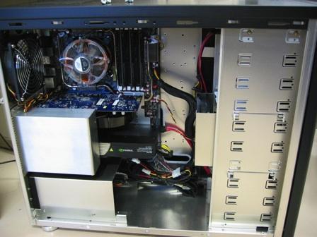
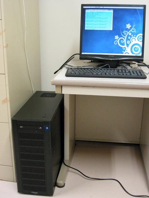
23 PIC solver in KEK-System A 3D Poisson solver Boundary condition in free space, φ( )=0. Green function Potential ϕ(r) = 1 4π 0 G(r) = 1 r G(r r )ρ(r )dr
24 Implementation Make Green function table G i,j,k = 1 x y z G(r) = 1 r xi + x/2 yj + y/2 zk + z/2 x i x/2 1 x2 + y 2 + z 2 dr = y j y/2 z k z/2 1 x2 + y 2 + z 2 dr x2 yz 2 tan 1 x y2 zx x 2 + y 2 + z 2 2 tan 1 y z2 xy x 2 + y 2 + z 2 2 tan 1 z x 2 + y 2 + z 2 +yz ln(x + x 2 + y 2 + z 2 )+zxln(y + x 2 + y 2 + z 2 )+xy ln(z + x 2 + y 2 + z 2 ) Calculate ρ array from macro particles distribution ρ i,j,k
25 ϕ(r) = 1 4π 0 Integration, convolution G(r r )ρ(r )dr = 1 4π 0 Direct summation Range of the suffix: i=1,nx, i-i =1-Nx,Nx-1 Since G-i,j,k=Gi,j.k, the G table size can be NxNyNz. i,j,k G i i,j j,k k ρ i,j,k
26 Solver using FFT G(k) = ρ(k) = G(r) exp(ik r)dr ρ(r) exp(ik r)dr Convolution ϕ(r) = 1 4π 0 1 (2π) 3 G(k)ρ(k) exp( ik r)dk
27 Discrete space G k = N xyz i=1 G(r i ) exp(ik r i ) G(r i )= 1 N xyz N xyz k=1 G k exp( ik r i ) ρ k = N xyz i=1 ρ(r i ) r exp(ik r i ) ρ(r i ) r = 1 N xyz N xyz i=1 ρ k exp( ik r i ) Convolution 4π 0 ϕ(r i )= j G(r i r j )ρ(r j ) r = 1 N xyz N xyz k=1 G k ρ k exp( ik r i )
28 Shifted Green function Mirror charge Mirror charge Green G m (r) = 1 r r 0 G i,j,k = 1 x y z xi + x/2 yj + y/2 zk + z/2 x i x/2 y j y/2 z k z/2 1 x2 + y 2 +(z z 0 ) 2 dr 1 x2 + y 2 +(z z 0 ) 2
29 Potential of Gaussian Charge distribution with σr=1mm Green: Charge distribution in free space Red: Charge distribution with mirror at x=0.035 mirror at free space 1/r (m mirror y=z= r = x (m)
. NVIDIA Tesla, 240 PU/GPU, 4GB memory Tesla performance 0.933TFlops/single precision and 78GFlops/double precision. KEK supercomputer SR11000, 0.")
30 GPGPU GPGPU - General Purpose computing on Graphical Processor Unit CUDA(NVIDIA), ATI Stream(ATI), OpenCL My machine: Core i7 PC with NVIDIA Tesla 1060 (500k yen). NVIDIA Tesla, 240 PU/GPU, 4GB memory Tesla performance 0.933TFlops/single precision and 78GFlops/double precision. KEK supercomputer SR11000, 0.13TFlops/Node.
31
32 3D particle-particle interaction Based on a Demo code: Fast N-Body Simulation with CUDA (L. Nyland, M. Harris, J. Prins, NVIDIA SDK) F i = e2 4π 0 j=i r ij ( r ij 2 + ε 2 ) 3/2 r ij = r i r j
33 CPU GPU GPU GPU CPU
34 H = P = ee(z) Ż = Reference frame P 2 c 2 + m 2 0 c4 e z 0 E(z )dz Pc 2 P 2 c 2 + m 2 0 c4 P = m 0 V 1 V 2 /c 2 P n = P n 1 + ee(z n 1 ) t V n = P n c 2 P 2 n + m 2 0 c4 Z n = Z n 1 + P n c 2 t P 2 n + m 2 0c4
35 Lorentz transformation Space charge r =...e H 0 e eez L(V 2 )e ϕ L 1 (V 2 ) e H 0 e eez L(V 1 )e ϕ L 1 (V 1 ) L 1 (V 2 )e eez e H 0 L(V 1 ) reference frame z, Δt Lorentz e H 0 e eez e ϕ r 0
36 Equation of motion in the reference frame v i,n = n e r e c 2 t N e /n e 1 Vn 2 /c 2 j=i r ij ( r ij 2 + ε 2 ) 3/2 n e : charge in a macro particle Particle motion is assumed to be non-relativistic in the reference frame.
37 Expression of L(V) L -1 (V1) e e R Edr e H 0 L(V2) v x,0 = v x 1 V 2 1 /c 2 1 V 1 v z /c 2 v y,0 = v y 1 V 2 1 /c 2 1 V 1 v z /c 2 v z,0 = v z V 1 1 V 1 v z /c 2 v x = v x,0 1 V 2 2 /c 2 1+V 2 v z,0 /c 2 v y = v y,0 1 V 2 2 /c 2 1+V 2 v z,0 /c 2 v z = v z,0 + V 2 1+V 2 v z,0 /c 2 z 0 = z V 1 t 1 V 2 1 /c 2 t 0 = t V 1z/c 2 1 V 2 1 /c 2 t 0 = t 1 V1 2/c2 z = z 0 + V 2 t 0 1 V 2 2 /c 2 t = t 0 + V 2 z 0 /c 2 1 V 2 2 /c 2
38 H = r p 2 c 2 + m 2 0 c4 e 0 H0 E(r )dr p n = p n 1 + ee(r n 1 ) t r n = r n 1 + p n c 2 t p 2 n c 2 + m 2 0c4
39 NVIDIA-Tesla: 30,000 ( 400GFlops sec/step. 100, sec/step ( N 2 ) Hitachi SR11000(KEK-SystemA), 3D-PIC 100, sec/step ( Blue Gene(KEK-SystemB)
untitled
 SPring-8 RFgun JASRI/SPring-8 6..7 Contents.. 3.. 5. 6. 7. 8. . 3 cavity γ E A = er 3 πε γ vb r B = v E c r c A B A ( ) F = e E + v B A A A A B dp e( v B+ E) = = m d dt dt ( γ v) dv e ( ) dt v B E v E
GPU GPU CPU CPU CPU GPU GPU N N CPU ( ) 1 GPU CPU GPU 2D 3D CPU GPU GPU GPGPU GPGPU 2 nvidia GPU CUDA 3 GPU 3.1 GPU Core 1
 1 GPU CPU GPU 2D 3D CPU GPU GPU GPGPU GPGPU 2 nvidia GPU CUDA 3 GPU 3.1 GPU Core 1") GPU 4 2010 8 28 1 GPU CPU CPU CPU GPU GPU N N CPU ( ) 1 GPU CPU GPU 2D 3D CPU GPU GPU GPGPU GPGPU 2 nvidia GPU CUDA 3 GPU 3.1 GPU Core 1 Register & Shared Memory ( ) CPU CPU(Intel Core i7 965) GPU(Tesla
GPU 4 2010 8 28 1 GPU CPU CPU CPU GPU GPU N N CPU ( ) 1 GPU CPU GPU 2D 3D CPU GPU GPU GPGPU GPGPU 2 nvidia GPU CUDA 3 GPU 3.1 GPU Core 1 Register & Shared Memory ( ) CPU CPU(Intel Core i7 965) GPU(Tesla
23 Fig. 2: hwmodulev2 3. Reconfigurable HPC 3.1 hw/sw hw/sw hw/sw FPGA PC FPGA PC FPGA HPC FPGA FPGA hw/sw hw/sw hw- Module FPGA hwmodule hw/sw FPGA h
 23 FPGA CUDA Performance Comparison of FPGA Array with CUDA on Poisson Equation ([email protected]), ([email protected]), ([email protected]), ([email protected]),
i
 009 I 1 8 5 i 0 1 0.1..................................... 1 0.................................................. 1 0.3................................. 0.4........................................... 3
m dv = mg + kv2 dt m dv dt = mg k v v m dv dt = mg + kv2 α = mg k v = α 1 e rt 1 + e rt m dv dt = mg + kv2 dv mg + kv 2 = dt m dv α 2 + v 2 = k m dt d
 m v = mg + kv m v = mg k v v m v = mg + kv α = mg k v = α e rt + e rt m v = mg + kv v mg + kv = m v α + v = k m v (v α (v + α = k m ˆ ( v α ˆ αk v = m v + α ln v α v + α = αk m t + C v α v + α = e αk m
 21 2 26 i 1 1 1.1............................ 1 1.2............................ 3 2 9 2.1................... 9 2.2.......... 9 2.3................... 11 2.4....................... 12 3 15 3.1..........
GPGPU
 GPGPU 2013 1008 2015 1 23 Abstract In recent years, with the advance of microscope technology, the alive cells have been able to observe. On the other hand, from the standpoint of image processing, the
Fourier series to Fourier transform Masahiro Yamamoto September 9, 2016 OB (r j)j r (r i)i Figure 1: normal coordinate, projection, inner product 3 r
j r (r i)i Figure 1: normal coordinate, projection, inner product 3 r") Fourier series to Fourier transform Masahiro Yamamoto September 9, 2016 OB (r j)j r (r i)i Figure 1: normal coordinate, projection, inner product 3 r i.j, k x = r i, y = r j, z = r k r = xi + yj + zk N
Fourier series to Fourier transform Masahiro Yamamoto September 9, 2016 OB (r j)j r (r i)i Figure 1: normal coordinate, projection, inner product 3 r i.j, k x = r i, y = r j, z = r k r = xi + yj + zk N
untitled
 A = QΛQ T A n n Λ Q A = XΛX 1 A n n Λ X GPGPU A 3 T Q T AQ = T (Q: ) T u i = λ i u i T {λ i } {u i } QR MR 3 v i = Q u i A {v i } A n = 9000 Quad Core Xeon 2 LAPACK (4/3) n 3 O(n 2 ) O(n 3 ) A {v i }
2 G(k) e ikx = (ik) n x n n! n=0 (k ) ( ) X n = ( i) n n k n G(k) k=0 F (k) ln G(k) = ln e ikx n κ n F (k) = F (k) (ik) n n= n! κ n κ n = ( i) n n k n
 e ikx = (ik) n x n n! n=0 (k ) ( ) X n = ( i) n n k n G(k) k=0 F (k) ln G(k) = ln e ikx n κ n F (k) = F (k) (ik) n n= n! κ n κ n = ( i) n n k n") . X {x, x 2, x 3,... x n } X X {, 2, 3, 4, 5, 6} X x i P i. 0 P i 2. n P i = 3. P (i ω) = i ω P i P 3 {x, x 2, x 3,... x n } ω P i = 6 X f(x) f(x) X n n f(x i )P i n x n i P i X n 2 G(k) e ikx = (ik) n
. X {x, x 2, x 3,... x n } X X {, 2, 3, 4, 5, 6} X x i P i. 0 P i 2. n P i = 3. P (i ω) = i ω P i P 3 {x, x 2, x 3,... x n } ω P i = 6 X f(x) f(x) X n n f(x i )P i n x n i P i X n 2 G(k) e ikx = (ik) n
Table 1: Basic parameter set. Aperture values indicate the radius. δ is relative momentum deviation. Parameter Value Unit Initial emittance 10 mm.mrad
 SuperKEKB EMITTANCE GROWTH BY MISALIGNMENTS AND JITTERS IN SUPERKEKB INJECTOR LINAC Y. Seimiya, M. Satoh, T. Suwada, T. Higo, Y. Enomoto, F. Miyahara, K. Furukawa High Energy Accelerator Research Organization
all.dvi
 5,, Euclid.,..,... Euclid,.,.,, e i (i =,, ). 6 x a x e e e x.:,,. a,,. a a = a e + a e + a e = {e, e, e } a (.) = a i e i = a i e i (.) i= {a,a,a } T ( T ),.,,,,. (.),.,...,,. a 0 0 a = a 0 + a + a 0
II 2 II
 II 2 II 2005 [email protected] 2005 4 1 1 2 5 2.1.................................... 5 2.2................................. 6 2.3............................. 6 2.4.................................
JKR Point loading of an elastic half-space 2 3 Pressure applied to a circular region Boussinesq, n =
 JKR 17 9 15 1 Point loading of an elastic half-space Pressure applied to a circular region 4.1 Boussinesq, n = 1.............................. 4. Hertz, n = 1.................................. 6 4 Hertz
n (1.6) i j=1 1 n a ij x j = b i (1.7) (1.7) (1.4) (1.5) (1.4) (1.7) u, v, w ε x, ε y, ε x, γ yz, γ zx, γ xy (1.8) ε x = u x ε y = v y ε z = w z γ yz
 i j=1 1 n a ij x j = b i (1.7) (1.7) (1.4) (1.5) (1.4) (1.7) u, v, w ε x, ε y, ε x, γ yz, γ zx, γ xy (1.8) ε x = u x ε y = v y ε z = w z γ yz") 1 2 (a 1, a 2, a n ) (b 1, b 2, b n ) A (1.1) A = a 1 b 1 + a 2 b 2 + + a n b n (1.1) n A = a i b i (1.2) i=1 n i 1 n i=1 a i b i n i=1 A = a i b i (1.3) (1.3) (1.3) (1.1) (ummation convention) a 11 x
1 2 (a 1, a 2, a n ) (b 1, b 2, b n ) A (1.1) A = a 1 b 1 + a 2 b 2 + + a n b n (1.1) n A = a i b i (1.2) i=1 n i 1 n i=1 a i b i n i=1 A = a i b i (1.3) (1.3) (1.3) (1.1) (ummation convention) a 11 x
液晶の物理1:連続体理論(弾性,粘性)
") The Physics of Liquid Crystals P. G. de Gennes and J. Prost (Oxford University Press, 1993) Liquid crystals are beautiful and mysterious; I am fond of them for both reasons. My hope is that some readers
The Physics of Liquid Crystals P. G. de Gennes and J. Prost (Oxford University Press, 1993) Liquid crystals are beautiful and mysterious; I am fond of them for both reasons. My hope is that some readers
5 1.2, 2, d a V a = M (1.2.1), M, a,,,,, Ω, V a V, V a = V + Ω r. (1.2.2), r i 1, i 2, i 3, i 1, i 2, i 3, A 2, A = 3 A n i n = n=1 da = 3 = n=1 3 n=1
, M, a,,,,, Ω, V a V, V a = V + Ω r. (1.2.2), r i 1, i 2, i 3, i 1, i 2, i 3, A 2, A = 3 A n i n = n=1 da = 3 = n=1 3 n=1") 4 1 1.1 ( ) 5 1.2, 2, d a V a = M (1.2.1), M, a,,,,, Ω, V a V, V a = V + Ω r. (1.2.2), r i 1, i 2, i 3, i 1, i 2, i 3, A 2, A = 3 A n i n = n=1 da = 3 = n=1 3 n=1 da n i n da n i n + 3 A ni n n=1 3 n=1
4 1 1.1 ( ) 5 1.2, 2, d a V a = M (1.2.1), M, a,,,,, Ω, V a V, V a = V + Ω r. (1.2.2), r i 1, i 2, i 3, i 1, i 2, i 3, A 2, A = 3 A n i n = n=1 da = 3 = n=1 3 n=1 da n i n da n i n + 3 A ni n n=1 3 n=1
4/15 No.
 4/15 No. 1 4/15 No. 4/15 No. 3 Particle of mass m moving in a potential V(r) V(r) m i ψ t = m ψ(r,t)+v(r)ψ(r,t) ψ(r,t) = ϕ(r)e iωt ψ(r,t) Wave function steady state m ϕ(r)+v(r)ϕ(r) = εϕ(r) Eigenvalue problem
07-二村幸孝・出口大輔.indd
 GPU Graphics Processing Units HPC High Performance Computing GPU GPGPU General-Purpose computation on GPU CPU GPU GPU *1 Intel Quad-Core Xeon E5472 3.0 GHz 2 6 MB L2 cache 1600 MHz FSB 80 GFlops 1 nvidia
( )
") 1. 2. 3. 4. 5. ( ) () http://www-astro.physics.ox.ac.uk/~wjs/apm_grey.gif http://antwrp.gsfc.nasa.gov/apod/ap950917.html ( ) SDSS : d 2 r i dt 2 = Gm jr ij j i rij 3 = Newton 3 0.1% 19 20 20 2 ( ) 3 3
1. 2. 3. 4. 5. ( ) () http://www-astro.physics.ox.ac.uk/~wjs/apm_grey.gif http://antwrp.gsfc.nasa.gov/apod/ap950917.html ( ) SDSS : d 2 r i dt 2 = Gm jr ij j i rij 3 = Newton 3 0.1% 19 20 20 2 ( ) 3 3
変 位 変位とは 物体中のある点が変形後に 別の点に異動したときの位置の変化で あり ベクトル量である 変位には 物体の変形の他に剛体運動 剛体変位 が含まれている 剛体変位 P(x, y, z) 平行移動と回転 P! (x + u, y + v, z + w) Q(x + d x, y + dy,
 平行移動と回転 P! (x + u, y + v, z + w) Q(x + d x, y + dy,") 変 位 変位とは 物体中のある点が変形後に 別の点に異動したときの位置の変化で あり ベクトル量である 変位には 物体の変形の他に剛体運動 剛体変位 が含まれている 剛体変位 P(x, y, z) 平行移動と回転 P! (x + u, y + v, z + w) Q(x + d x, y + dy, z + dz) Q! (x + d x + u + du, y + dy + v + dv, z +
変 位 変位とは 物体中のある点が変形後に 別の点に異動したときの位置の変化で あり ベクトル量である 変位には 物体の変形の他に剛体運動 剛体変位 が含まれている 剛体変位 P(x, y, z) 平行移動と回転 P! (x + u, y + v, z + w) Q(x + d x, y + dy, z + dz) Q! (x + d x + u + du, y + dy + v + dv, z +
.5 z = a + b + c n.6 = a sin t y = b cos t dy d a e e b e + e c e e e + e 3 s36 3 a + y = a, b > b 3 s363.7 y = + 3 y = + 3 s364.8 cos a 3 s365.9 y =,
 [ ] IC. r, θ r, θ π, y y = 3 3 = r cos θ r sin θ D D = {, y ; y }, y D r, θ ep y yddy D D 9 s96. d y dt + 3dy + y = cos t dt t = y = e π + e π +. t = π y =.9 s6.3 d y d + dy d + y = y =, dy d = 3 a, b
1 GPU GPGPU GPU CPU 2 GPU 2007 NVIDIA GPGPU CUDA[3] GPGPU CUDA GPGPU CUDA GPGPU GPU GPU GPU Graphics Processing Unit LSI LSI CPU ( ) DRAM GPU LSI GPU
![1 GPU GPGPU GPU CPU 2 GPU 2007 NVIDIA GPGPU CUDA[3] GPGPU CUDA GPGPU CUDA GPGPU GPU GPU GPU Graphics Processing Unit LSI LSI CPU ( ) DRAM GPU LSI GPU](/thumbs/89/99132402.jpg "1 GPU GPGPU GPU CPU 2 GPU 2007 NVIDIA GPGPU CUDA[3] GPGPU CUDA GPGPU CUDA GPGPU GPU GPU GPU Graphics Processing Unit LSI LSI CPU ( ) DRAM GPU LSI GPU") GPGPU (I) GPU GPGPU 1 GPU(Graphics Processing Unit) GPU GPGPU(General-Purpose computing on GPUs) GPU GPGPU GPU ( PC ) PC PC GPU PC PC GPU GPU 2008 TSUBAME NVIDIA GPU(Tesla S1070) TOP500 29 [1] 2009 AMD
GPGPU (I) GPU GPGPU 1 GPU(Graphics Processing Unit) GPU GPGPU(General-Purpose computing on GPUs) GPU GPGPU GPU ( PC ) PC PC GPU PC PC GPU GPU 2008 TSUBAME NVIDIA GPU(Tesla S1070) TOP500 29 [1] 2009 AMD
Part () () Γ Part ,
 () Γ Part ,") Contents a 6 6 6 6 6 6 6 7 7. 8.. 8.. 8.3. 8 Part. 9. 9.. 9.. 3. 3.. 3.. 3 4. 5 4.. 5 4.. 9 4.3. 3 Part. 6 5. () 6 5.. () 7 5.. 9 5.3. Γ 3 6. 3 6.. 3 6.. 3 6.3. 33 Part 3. 34 7. 34 7.. 34 7.. 34 8. 35
Contents a 6 6 6 6 6 6 6 7 7. 8.. 8.. 8.3. 8 Part. 9. 9.. 9.. 3. 3.. 3.. 3 4. 5 4.. 5 4.. 9 4.3. 3 Part. 6 5. () 6 5.. () 7 5.. 9 5.3. Γ 3 6. 3 6.. 3 6.. 3 6.3. 33 Part 3. 34 7. 34 7.. 34 7.. 34 8. 35
2.2 h h l L h L = l cot h (1) (1) L l L l l = L tan h (2) (2) L l 2 l 3 h 2.3 a h a h (a, h)
 (1) L l L l l = L tan h (2) (2) L l 2 l 3 h 2.3 a h a h (a, h)") 1 16 10 5 1 2 2.1 a a a 1 1 1 2.2 h h l L h L = l cot h (1) (1) L l L l l = L tan h (2) (2) L l 2 l 3 h 2.3 a h a h (a, h) 4 2 3 4 2 5 2.4 x y (x,y) l a x = l cot h cos a, (3) y = l cot h sin a (4) h a
1 16 10 5 1 2 2.1 a a a 1 1 1 2.2 h h l L h L = l cot h (1) (1) L l L l l = L tan h (2) (2) L l 2 l 3 h 2.3 a h a h (a, h) 4 2 3 4 2 5 2.4 x y (x,y) l a x = l cot h cos a, (3) y = l cot h sin a (4) h a
MUFFIN3
 MUFFIN - MUltiFarious FIeld simulator for Non-equilibrium system - ( ) MUFFIN WG3 - - JCII, - ( ) - ( ) - ( ) - (JSR) - - MUFFIN sec -3 msec -6 sec GOURMET SUSHI MUFFIN -9 nsec PASTA -1 psec -15 fsec COGNAC
AMD/ATI Radeon HD 5870 GPU DEGIMA LINPACK HD 5870 GPU DEGIMA LINPACK GFlops/Watt GFlops/Watt Abstract GPU Computing has lately attracted
 DEGIMA LINPACK Energy Performance for LINPACK Benchmark on DEGIMA 1 AMD/ATI Radeon HD 5870 GPU DEGIMA LINPACK HD 5870 GPU DEGIMA LINPACK 1.4698 GFlops/Watt 1.9658 GFlops/Watt Abstract GPU Computing has
80 4 r ˆρ i (r, t) δ(r x i (t)) (4.1) x i (t) ρ i ˆρ i t = 0 i r 0 t(> 0) j r 0 + r < δ(r 0 x i (0))δ(r 0 + r x j (t)) > (4.2) r r 0 G i j (r, t) dr 0
 δ(r x i (t)) (4.1) x i (t) ρ i ˆρ i t = 0 i r 0 t(> 0) j r 0 + r < δ(r 0 x i (0))δ(r 0 + r x j (t)) > (4.2) r r 0 G i j (r, t) dr 0") 79 4 4.1 4.1.1 x i (t) x j (t) O O r 0 + r r r 0 x i (0) r 0 x i (0) 4.1 L. van. Hove 1954 space-time correlation function V N 4.1 ρ 0 = N/V i t 80 4 r ˆρ i (r, t) δ(r x i (t)) (4.1) x i (t) ρ i ˆρ i t
79 4 4.1 4.1.1 x i (t) x j (t) O O r 0 + r r r 0 x i (0) r 0 x i (0) 4.1 L. van. Hove 1954 space-time correlation function V N 4.1 ρ 0 = N/V i t 80 4 r ˆρ i (r, t) δ(r x i (t)) (4.1) x i (t) ρ i ˆρ i t
all.dvi
 38 5 Cauchy.,,,,., σ.,, 3,,. 5.1 Cauchy (a) (b) (a) (b) 5.1: 5.1. Cauchy 39 F Q Newton F F F Q F Q 5.2: n n ds df n ( 5.1). df n n df(n) df n, t n. t n = df n (5.1) ds 40 5 Cauchy t l n mds df n 5.3: t
( )/2 hara/lectures/lectures-j.html 2, {H} {T } S = {H, T } {(H, H), (H, T )} {(H, T ), (T, T )} {(H, H), (T, T )} {1
/2 hara/lectures/lectures-j.html 2, {H} {T } S = {H, T } {(H, H), (H, T )} {(H, T ), (T, T )} {(H, H), (T, T )} {1") ( )/2 http://www2.math.kyushu-u.ac.jp/ hara/lectures/lectures-j.html 1 2011 ( )/2 2 2011 4 1 2 1.1 1 2 1 2 3 4 5 1.1.1 sample space S S = {H, T } H T T H S = {(H, H), (H, T ), (T, H), (T, T )} (T, H) S
( )/2 http://www2.math.kyushu-u.ac.jp/ hara/lectures/lectures-j.html 1 2011 ( )/2 2 2011 4 1 2 1.1 1 2 1 2 3 4 5 1.1.1 sample space S S = {H, T } H T T H S = {(H, H), (H, T ), (T, H), (T, T )} (T, H) S
sec13.dvi
 13 13.1 O r F R = m d 2 r dt 2 m r m = F = m r M M d2 R dt 2 = m d 2 r dt 2 = F = F (13.1) F O L = r p = m r ṙ dl dt = m ṙ ṙ + m r r = r (m r ) = r F N. (13.2) N N = R F 13.2 O ˆn ω L O r u u = ω r 1 1:
 2005 2006.2.22-1 - 1 Fig. 1 2005 2006.2.22-2 - Element-Free Galerkin Method (EFGM) Meshless Local Petrov-Galerkin Method (MLPGM) 2005 2006.2.22-3 - 2 MLS u h (x) 1 p T (x) = [1, x, y]. (1) φ(x) 0.5 φ(x)
! 行行 CPUDSP PPESPECell/B.E. CPUGPU 行行 SIMD [SSE, AltiVec] 用 HPC CPUDSP PPESPE (Cell/B.E.) SPE CPUGPU GPU CPU DSP DSP PPE SPE SPE CPU DSP SPE 2
![! 行行 CPUDSP PPESPECell/B.E. CPUGPU 行行 SIMD [SSE, AltiVec] 用 HPC CPUDSP PPESPE (Cell/B.E.) SPE CPUGPU GPU CPU DSP DSP PPE SPE SPE CPU DSP SPE 2](/thumbs/88/115445009.jpg "! 行行 CPUDSP PPESPECell/B.E. CPUGPU 行行 SIMD [SSE, AltiVec] 用 HPC CPUDSP PPESPE (Cell/B.E.) SPE CPUGPU GPU CPU DSP DSP PPE SPE SPE CPU DSP SPE 2") ! OpenCL [Open Computing Language] 言 [OpenCL C 言 ] CPU, GPU, Cell/B.E.,DSP 言 行行 [OpenCL Runtime] OpenCL C 言 API Khronos OpenCL Working Group AMD Broadcom Blizzard Apple ARM Codeplay Electronic Arts Freescale
! OpenCL [Open Computing Language] 言 [OpenCL C 言 ] CPU, GPU, Cell/B.E.,DSP 言 行行 [OpenCL Runtime] OpenCL C 言 API Khronos OpenCL Working Group AMD Broadcom Blizzard Apple ARM Codeplay Electronic Arts Freescale
Microsoft PowerPoint - 島田美帆.ppt
 コンパクト ERL におけるバンチ圧縮の可能性に関して 分子科学研究所,UVSOR 島田美帆日本原子力研究開発機構,JAEA 羽島良一 Outline Beam dynamics studies for the 5 GeV ERL 規格化エミッタンス 0.1 mm mrad を維持する周回部の設計 Towards user experiment at the compact ERL Short bunch
main.dvi
 PC 1 1 [1][2] [3][4] ( ) GPU(Graphics Processing Unit) GPU PC GPU PC ( 2 GPU ) GPU Harris Corner Detector[5] CPU ( ) ( ) CPU GPU 2 3 GPU 4 5 6 7 1 [email protected] 45 2 ( ) CPU ( ) ( ) () 2.1
The Physics of Atmospheres CAPTER :
 The Physics of Atmospheres CAPTER 4 1 4 2 41 : 2 42 14 43 17 44 25 45 27 46 3 47 31 48 32 49 34 41 35 411 36 maintex 23/11/28 The Physics of Atmospheres CAPTER 4 2 4 41 : 2 1 σ 2 (21) (22) k I = I exp(
2.5 (Gauss) (flux) v(r)( ) S n S v n v n (1) v n S = v n S = v S, n S S. n n S v S v Minoru TANAKA (Osaka Univ.) I(2012), Sec p. 1/30
 (flux) v(r)( ) S n S v n v n (1) v n S = v n S = v S, n S S. n n S v S v Minoru TANAKA (Osaka Univ.) I(2012), Sec p. 1/30") 2.5 (Gauss) 2.5.1 (flux) v(r)( ) n v n v n (1) v n = v n = v, n. n n v v I(2012), ec. 2. 5 p. 1/30 i (2) lim v(r i ) i = v(r) d. i 0 i (flux) I(2012), ec. 2. 5 p. 2/30 2.5.2 ( ) ( ) q 1 r 2 E 2 q r 1 E
2.5 (Gauss) 2.5.1 (flux) v(r)( ) n v n v n (1) v n = v n = v, n. n n v v I(2012), ec. 2. 5 p. 1/30 i (2) lim v(r i ) i = v(r) d. i 0 i (flux) I(2012), ec. 2. 5 p. 2/30 2.5.2 ( ) ( ) q 1 r 2 E 2 q r 1 E
50 2 I SI MKSA r q r q F F = 1 qq 4πε 0 r r 2 r r r r (2.2 ε 0 = 1 c 2 µ 0 c = m/s q 2.1 r q' F r = 0 µ 0 = 4π 10 7 N/A 2 k = 1/(4πε 0 qq
 49 2 I II 2.1 3 e e = 1.602 10 19 A s (2.1 50 2 I SI MKSA 2.1.1 r q r q F F = 1 qq 4πε 0 r r 2 r r r r (2.2 ε 0 = 1 c 2 µ 0 c = 3 10 8 m/s q 2.1 r q' F r = 0 µ 0 = 4π 10 7 N/A 2 k = 1/(4πε 0 qq F = k r
IPSJ SIG Technical Report Vol.2013-ARC-203 No /2/1 SMYLE OpenCL (NEDO) IT FPGA SMYLEref SMYLE OpenCL SMYLE OpenCL FPGA 1
 IT FPGA SMYLEref SMYLE OpenCL SMYLE OpenCL FPGA 1") SMYLE OpenCL 128 1 1 1 1 1 2 2 3 3 3 (NEDO) IT FPGA SMYLEref SMYLE OpenCL SMYLE OpenCL FPGA 128 SMYLEref SMYLE OpenCL SMYLE OpenCL Implementation and Evaluations on 128 Cores Takuji Hieda 1 Noriko Etani
SMYLE OpenCL 128 1 1 1 1 1 2 2 3 3 3 (NEDO) IT FPGA SMYLEref SMYLE OpenCL SMYLE OpenCL FPGA 128 SMYLEref SMYLE OpenCL SMYLE OpenCL Implementation and Evaluations on 128 Cores Takuji Hieda 1 Noriko Etani
 006 11 8 0 3 1 5 1.1..................... 5 1......................... 6 1.3.................... 6 1.4.................. 8 1.5................... 8 1.6................... 10 1.6.1......................
2 Chapter 4 (f4a). 2. (f4cone) ( θ) () g M. 2. (f4b) T M L P a θ (f4eki) ρ H A a g. v ( ) 2. H(t) ( )
. 2. (f4cone) ( θ) () g M. 2. (f4b) T M L P a θ (f4eki) ρ H A a g. v ( ) 2. H(t) ( )") http://astr-www.kj.yamagata-u.ac.jp/~shibata f4a f4b 2 f4cone f4eki f4end 4 f5meanfp f6coin () f6a f7a f7b f7d f8a f8b f9a f9b f9c f9kep f0a f0bt version feqmo fvec4 fvec fvec6 fvec2 fvec3 f3a (-D) f3b
http://astr-www.kj.yamagata-u.ac.jp/~shibata f4a f4b 2 f4cone f4eki f4end 4 f5meanfp f6coin () f6a f7a f7b f7d f8a f8b f9a f9b f9c f9kep f0a f0bt version feqmo fvec4 fvec fvec6 fvec2 fvec3 f3a (-D) f3b
No δs δs = r + δr r = δr (3) δs δs = r r = δr + u(r + δr, t) u(r, t) (4) δr = (δx, δy, δz) u i (r + δr, t) u i (r, t) = u i x j δx j (5) δs 2
 δs δs = r r = δr + u(r + δr, t) u(r, t) (4) δr = (δx, δy, δz) u i (r + δr, t) u i (r, t) = u i x j δx j (5) δs 2") No.2 1 2 2 δs δs = r + δr r = δr (3) δs δs = r r = δr + u(r + δr, t) u(r, t) (4) δr = (δx, δy, δz) u i (r + δr, t) u i (r, t) = u i δx j (5) δs 2 = δx i δx i + 2 u i δx i δx j = δs 2 + 2s ij δx i δx j
No.2 1 2 2 δs δs = r + δr r = δr (3) δs δs = r r = δr + u(r + δr, t) u(r, t) (4) δr = (δx, δy, δz) u i (r + δr, t) u i (r, t) = u i δx j (5) δs 2 = δx i δx i + 2 u i δx i δx j = δs 2 + 2s ij δx i δx j
OHO.dvi
 1 Coil D-shaped electrodes ( [1] ) Vacuum chamber Ion source Oscillator 1.1 m e v B F = evb (1) r m v2 = evb r v = erb (2) m r T = 2πr v = 2πm (3) eb v
GPU n Graphics Processing Unit CG CAD
 GPU 2016/06/27 第 20 回 GPU コンピューティング講習会 ( 東京工業大学 ) 1 GPU n Graphics Processing Unit CG CAD www.nvidia.co.jp www.autodesk.co.jp www.pixar.com GPU n GPU ü n NVIDIA CUDA ü NVIDIA GPU ü OS Linux, Windows, Mac
Gmech08.dvi
 145 13 13.1 13.1.1 0 m mg S 13.1 F 13.1 F /m S F F 13.1 F mg S F F mg 13.1: m d2 r 2 = F + F = 0 (13.1) 146 13 F = F (13.2) S S S S S P r S P r r = r 0 + r (13.3) r 0 S S m d2 r 2 = F (13.4) (13.3) d 2
all.dvi
 72 9 Hooke,,,. Hooke. 9.1 Hooke 1 Hooke. 1, 1 Hooke. σ, ε, Young. σ ε (9.1), Young. τ γ G τ Gγ (9.2) X 1, X 2. Poisson, Poisson ν. ν ε 22 (9.) ε 11 F F X 2 X 1 9.1: Poisson 9.1. Hooke 7 Young Poisson G
I ( ) 1 de Broglie 1 (de Broglie) p λ k h Planck ( Js) p = h λ = k (1) h 2π : Dirac k B Boltzmann ( J/K) T U = 3 2 k BT
 1 de Broglie 1 (de Broglie) p λ k h Planck ( Js) p = h λ = k (1) h 2π : Dirac k B Boltzmann ( J/K) T U = 3 2 k BT") I (008 4 0 de Broglie (de Broglie p λ k h Planck ( 6.63 0 34 Js p = h λ = k ( h π : Dirac k B Boltzmann (.38 0 3 J/K T U = 3 k BT ( = λ m k B T h m = 0.067m 0 m 0 = 9. 0 3 kg GaAs( a T = 300 K 3 fg 07345
I (008 4 0 de Broglie (de Broglie p λ k h Planck ( 6.63 0 34 Js p = h λ = k ( h π : Dirac k B Boltzmann (.38 0 3 J/K T U = 3 k BT ( = λ m k B T h m = 0.067m 0 m 0 = 9. 0 3 kg GaAs( a T = 300 K 3 fg 07345
GPUを用いたN体計算
 単精度 190Tflops GPU クラスタ ( 長崎大 ) の紹介 長崎大学工学部超高速メニーコアコンピューティングセンターテニュアトラック助教濱田剛 1 概要 GPU (Graphics Processing Unit) について簡単に説明します. GPU クラスタが得意とする応用問題を議論し 長崎大学での GPU クラスタによる 取組方針 N 体計算の高速化に関する研究内容 を紹介します. まとめ
 n ξ n,i, i = 1,, n S n ξ n,i n 0 R 1,.. σ 1 σ i .10.14.15 0 1 0 1 1 3.14 3.18 3.19 3.14 3.14,. ii 1 1 1.1..................................... 1 1............................... 3 1.3.........................
Agenda GRAPE-MPの紹介と性能評価 GRAPE-MPの概要 OpenCLによる四倍精度演算 (preliminary) 4倍精度演算用SIM 加速ボード 6 processor elem with 128 bit logic Peak: 1.2Gflops
 4倍精度演算用SIM 加速ボード 6 processor elem with 128 bit logic Peak: 1.2Gflops") Agenda GRAPE-MPの紹介と性能評価 GRAPE-MPの概要 OpenCLによる四倍精度演算 (preliminary) 4倍精度演算用SIM 加速ボード 6 processor elem with 128 bit logic Peak: 1.2Gflops ボードの概要 Control processor (FPGA by Altera) GRAPE-MP chip[nextreme
Agenda GRAPE-MPの紹介と性能評価 GRAPE-MPの概要 OpenCLによる四倍精度演算 (preliminary) 4倍精度演算用SIM 加速ボード 6 processor elem with 128 bit logic Peak: 1.2Gflops ボードの概要 Control processor (FPGA by Altera) GRAPE-MP chip[nextreme
AHPを用いた大相撲の新しい番付編成
 5304050 2008/2/15 1 2008/2/15 2 42 2008/2/15 3 2008/2/15 4 195 2008/2/15 5 2008/2/15 6 i j ij >1 ij ij1/>1 i j i 1 ji 1/ j ij 2008/2/15 7 1 =2.01/=0.5 =1.51/=0.67 2008/2/15 8 1 2008/2/15 9 () u ) i i i
 IA [email protected] Last updated: January,......................................................................................................................................................................................
W u = u(x, t) u tt = a 2 u xx, a > 0 (1) D := {(x, t) : 0 x l, t 0} u (0, t) = 0, u (l, t) = 0, t 0 (2)
 u tt = a 2 u xx, a > 0 (1) D := {(x, t) : 0 x l, t 0} u (0, t) = 0, u (l, t) = 0, t 0 (2)") 3 215 4 27 1 1 u u(x, t) u tt a 2 u xx, a > (1) D : {(x, t) : x, t } u (, t), u (, t), t (2) u(x, ) f(x), u(x, ) t 2, x (3) u(x, t) X(x)T (t) u (1) 1 T (t) a 2 T (t) X (x) X(x) α (2) T (t) αa 2 T (t) (4)
3 215 4 27 1 1 u u(x, t) u tt a 2 u xx, a > (1) D : {(x, t) : x, t } u (, t), u (, t), t (2) u(x, ) f(x), u(x, ) t 2, x (3) u(x, t) X(x)T (t) u (1) 1 T (t) a 2 T (t) X (x) X(x) α (2) T (t) αa 2 T (t) (4)
k m m d2 x i dt 2 = f i = kx i (i = 1, 2, 3 or x, y, z) f i σ ij x i e ij = 2.1 Hooke s law and elastic constants (a) x i (2.1) k m σ A σ σ σ σ f i x
 f i σ ij x i e ij = 2.1 Hooke s law and elastic constants (a) x i (2.1) k m σ A σ σ σ σ f i x") k m m d2 x i dt 2 = f i = kx i (i = 1, 2, 3 or x, y, z) f i ij x i e ij = 2.1 Hooke s law and elastic constants (a) x i (2.1) k m A f i x i B e e e e 0 e* e e (2.1) e (b) A e = 0 B = 0 (c) (2.1) (d) e
k m m d2 x i dt 2 = f i = kx i (i = 1, 2, 3 or x, y, z) f i ij x i e ij = 2.1 Hooke s law and elastic constants (a) x i (2.1) k m A f i x i B e e e e 0 e* e e (2.1) e (b) A e = 0 B = 0 (c) (2.1) (d) e
120 9 I I 1 I 2 I 1 I 2 ( a) ( b) ( c ) I I 2 I 1 I ( d) ( e) ( f ) 9.1: Ampère (c) (d) (e) S I 1 I 2 B ds = µ 0 ( I 1 I 2 ) I 1 I 2 B ds =0. I 1 I 2
 ( b) ( c ) I I 2 I 1 I ( d) ( e) ( f ) 9.1: Ampère (c) (d) (e) S I 1 I 2 B ds = µ 0 ( I 1 I 2 ) I 1 I 2 B ds =0. I 1 I 2") 9 E B 9.1 9.1.1 Ampère Ampère Ampère s law B S µ 0 B ds = µ 0 j ds (9.1) S rot B = µ 0 j (9.2) S Ampère Biot-Savart oulomb Gauss Ampère rot B 0 Ampère µ 0 9.1 (a) (b) I B ds = µ 0 I. I 1 I 2 B ds = µ 0
9 E B 9.1 9.1.1 Ampère Ampère Ampère s law B S µ 0 B ds = µ 0 j ds (9.1) S rot B = µ 0 j (9.2) S Ampère Biot-Savart oulomb Gauss Ampère rot B 0 Ampère µ 0 9.1 (a) (b) I B ds = µ 0 I. I 1 I 2 B ds = µ 0
スライド 1
 Matsuura Laboratory SiC SiC 13 2004 10 21 22 H-SiC ( C-SiC HOY Matsuura Laboratory n E C E D ( E F E T Matsuura Laboratory Matsuura Laboratory DLTS Osaka Electro-Communication University Unoped n 3C-SiC

 B 1 B.1.......................... 1 B.1.1................. 1 B.1.2................. 2 B.2........................... 5 B.2.1.......................... 5 B.2.2.................. 6 B.2.3..................
 20 6 4 1 4 1.1 1.................................... 4 1.1.1.................................... 4 1.1.2 1................................ 5 1.2................................... 7 1.2.1....................................
1 I 1.1 ± e = = - = C C MKSA [m], [Kg] [s] [A] 1C 1A 1 MKSA 1C 1C +q q +q q 1
![1 I 1.1 ± e = = - = C C MKSA [m], [Kg] [s] [A] 1C 1A 1 MKSA 1C 1C +q q +q q 1](/thumbs/94/121802164.jpg "1 I 1.1 ± e = = - = C C MKSA [m], [Kg] [s] [A] 1C 1A 1 MKSA 1C 1C +q q +q q 1") 1 I 1.1 ± e = = - =1.602 10 19 C C MKA [m], [Kg] [s] [A] 1C 1A 1 MKA 1C 1C +q q +q q 1 1.1 r 1,2 q 1, q 2 r 12 2 q 1, q 2 2 F 12 = k q 1q 2 r 12 2 (1.1) k 2 k 2 ( r 1 r 2 ) ( r 2 r 1 ) q 1 q 2 (q 1 q 2
1 I 1.1 ± e = = - =1.602 10 19 C C MKA [m], [Kg] [s] [A] 1C 1A 1 MKA 1C 1C +q q +q q 1 1.1 r 1,2 q 1, q 2 r 12 2 q 1, q 2 2 F 12 = k q 1q 2 r 12 2 (1.1) k 2 k 2 ( r 1 r 2 ) ( r 2 r 1 ) q 1 q 2 (q 1 q 2
PowerPoint Presentation
 2010 KEK (Japan) (Japan) (Japan) Cheoun, Myun -ki Soongsil (Korea) Ryu,, Chung-Yoe Soongsil (Korea) 1. S.Reddy, M.Prakash and J.M. Lattimer, P.R.D58 #013009 (1998) Magnetar : ~ 10 15 G ~ 10 17 19 G (?)
(2 X Poisso P (λ ϕ X (t = E[e itx ] = k= itk λk e k! e λ = (e it λ k e λ = e eitλ e λ = e λ(eit 1. k! k= 6.7 X N(, 1 ϕ X (t = e 1 2 t2 : Cauchy ϕ X (t
![(2 X Poisso P (λ ϕ X (t = E[e itx ] = k= itk λk e k! e λ = (e it λ k e λ = e eitλ e λ = e λ(eit 1. k! k= 6.7 X N(, 1 ϕ X (t = e 1 2 t2 : Cauchy ϕ X (t](/thumbs/67/56612994.jpg "(2 X Poisso P (λ ϕ X (t = E[e itx ] = k= itk λk e k! e λ = (e it λ k e λ = e eitλ e λ = e λ(eit 1. k! k= 6.7 X N(, 1 ϕ X (t = e 1 2 t2 : Cauchy ϕ X (t") 6 6.1 6.1 (1 Z ( X = e Z, Y = Im Z ( Z = X + iy, i = 1 (2 Z E[ e Z ] < E[ Im Z ] < Z E[Z] = E[e Z] + ie[im Z] 6.2 Z E[Z] E[ Z ] : E[ Z ] < e Z Z, Im Z Z E[Z] α = E[Z], Z = Z Z 1 {Z } E[Z] = α = α [ α ]
6 6.1 6.1 (1 Z ( X = e Z, Y = Im Z ( Z = X + iy, i = 1 (2 Z E[ e Z ] < E[ Im Z ] < Z E[Z] = E[e Z] + ie[im Z] 6.2 Z E[Z] E[ Z ] : E[ Z ] < e Z Z, Im Z Z E[Z] α = E[Z], Z = Z Z 1 {Z } E[Z] = α = α [ α ]
‚åŁÎ“·„´Šš‡ðŠp‡¢‡½‹âfi`fiI…A…‰…S…−…Y…•‡ÌMarkovŸA“½fiI›ð’Í
 Markov 2009 10 2 Markov 2009 10 2 1 / 25 1 (GA) 2 GA 3 4 Markov 2009 10 2 2 / 25 (GA) (GA) L ( 1) I := {0, 1} L f : I (0, ) M( 2) S := I M GA (GA) f (i) i I Markov 2009 10 2 3 / 25 (GA) ρ(i, j), i, j I
LLG-R8.Nisus.pdf
 d M d t = γ M H + α M d M d t M γ [ 1/ ( Oe sec) ] α γ γ = gµ B h g g µ B h / π γ g = γ = 1.76 10 [ 7 1/ ( Oe sec) ] α α = λ γ λ λ λ α γ α α H α = γ H ω ω H α α H K K H K / M 1 1 > 0 α 1 M > 0 γ α γ =
2.4 ( ) ( B ) A B F (1) W = B A F dr. A F q dr f(x,y,z) A B Γ( ) Minoru TANAKA (Osaka Univ.) I(2011), Sec p. 1/30
 ( B ) A B F (1) W = B A F dr. A F q dr f(x,y,z) A B Γ( ) Minoru TANAKA (Osaka Univ.) I(2011), Sec p. 1/30") 2.4 ( ) 2.4.1 ( B ) A B F (1) W = B A F dr. A F q dr f(x,y,z) A B Γ( ) I(2011), Sec. 2. 4 p. 1/30 (2) Γ f dr lim f i r i. r i 0 i f i i f r i i i+1 (1) n i r i (3) F dr = lim F i n i r i. Γ r i 0 i n i
2.4 ( ) 2.4.1 ( B ) A B F (1) W = B A F dr. A F q dr f(x,y,z) A B Γ( ) I(2011), Sec. 2. 4 p. 1/30 (2) Γ f dr lim f i r i. r i 0 i f i i f r i i i+1 (1) n i r i (3) F dr = lim F i n i r i. Γ r i 0 i n i
1 (1) () (3) I 0 3 I I d θ = L () dt θ L L θ I d θ = L = κθ (3) dt κ T I T = π κ (4) T I κ κ κ L l a θ L r δr δl L θ ϕ ϕ = rθ (5) l
 () (3) I 0 3 I I d θ = L () dt θ L L θ I d θ = L = κθ (3) dt κ T I T = π κ (4) T I κ κ κ L l a θ L r δr δl L θ ϕ ϕ = rθ (5) l") 1 1 ϕ ϕ ϕ S F F = ϕ (1) S 1: F 1 1 (1) () (3) I 0 3 I I d θ = L () dt θ L L θ I d θ = L = κθ (3) dt κ T I T = π κ (4) T I κ κ κ L l a θ L r δr δl L θ ϕ ϕ = rθ (5) l : l r δr θ πrδr δf (1) (5) δf = ϕ πrδr
1 1 ϕ ϕ ϕ S F F = ϕ (1) S 1: F 1 1 (1) () (3) I 0 3 I I d θ = L () dt θ L L θ I d θ = L = κθ (3) dt κ T I T = π κ (4) T I κ κ κ L l a θ L r δr δl L θ ϕ ϕ = rθ (5) l : l r δr θ πrδr δf (1) (5) δf = ϕ πrδr
Microsoft PowerPoint - GPU_computing_2013_01.pptx
 GPU コンピューティン No.1 導入 東京工業大学 学術国際情報センター 青木尊之 1 GPU とは 2 GPGPU (General-purpose computing on graphics processing units) GPU を画像処理以外の一般的計算に使う GPU の魅力 高性能 : ハイエンド GPU はピーク 4 TFLOPS 超 手軽さ : 普通の PC にも装着できる 低価格
 iphone GPGPU GPU OpenCL Mac OS X Snow LeopardOpenCL iphone OpenCL OpenCL NVIDIA GPU CUDA GPU GPU GPU 15 GPU GPU CPU GPU iii OpenMP MPI CPU OpenCL CUDA OpenCL CPU OpenCL GPU NVIDIA Fermi GPU Fermi GPU GPU
cm λ λ = h/p p ( ) λ = cm E pc [ev] 2.2 quark lepton u d c s t b e 1 3e electric charge e color charge red blue green qq
![cm λ λ = h/p p ( ) λ = cm E pc [ev] 2.2 quark lepton u d c s t b e 1 3e electric charge e color charge red blue green qq](/thumbs/89/98710373.jpg "cm λ λ = h/p p ( ) λ = cm E pc [ev] 2.2 quark lepton u d c s t b e 1 3e electric charge e color charge red blue green qq") 2007 2007 7 1. 2. 3. 4. 5. 6. 7. 8. 9. 10. 1 2007 2 4 5 6 6 2 2.1 1: KEK Web page 1 1 1 10 16 cm λ λ = h/p p ( ) λ = 10 16 cm E pc [ev] 2.2 quark lepton 2 2.2.1 u d c s t b + 2 3 e 1 3e electric charge
2007 2007 7 1. 2. 3. 4. 5. 6. 7. 8. 9. 10. 1 2007 2 4 5 6 6 2 2.1 1: KEK Web page 1 1 1 10 16 cm λ λ = h/p p ( ) λ = 10 16 cm E pc [ev] 2.2 quark lepton 2 2.2.1 u d c s t b + 2 3 e 1 3e electric charge
JFE.dvi
 ,, Department of Civil Engineering, Chuo University Kasuga 1-13-27, Bunkyo-ku, Tokyo 112 8551, JAPAN E-mail : [email protected] E-mail : [email protected] SATO KOGYO CO., LTD. 12-20, Nihonbashi-Honcho