COGNACのコンセプト \(COarse Grained molecular dynamics program developed by NAgoya Cooperation\)
|
|
|
- みさえ おとじま
- 8 years ago
- Views:
Transcription
1 COGNAC (COarse-Grained molecular dynamics program by NAgoya Cooperation) ( ),
2 0 sec -3 msec -6 sec -9 nsec -12 psec -15 fsec GOURMET SUSHI PASTA COGNAC MUFFIN fm pm nm m mm m
3 United atom model (CH 2 ) Gay-Berne potential model Bead-spring model
4
5 Molecular dynamics (MD) Ensembles»NVE» NVT,NPH,NPT (loose-coupling / extended Hamiltonian methods) Langevin dynamics Molecular mechanics (MM) Steepest descent / conjugate gradient methods
6 Bonding 2-body(bond):Harmonic,Morse,FENE,Gaussian, Polynomial,Table 3-body(angle):Theta harmonic,cosine harmonic Theta polynomial,table 4-body(torsion):Cosine polynomial,table Non-bonding pair interaction Lennard-Jones,Gay-Berne,LJ-GB, Table Electrostatic Coulomb interaction(ewald,reaction field) Dipole-dipole interaction (Reaction field)

 Nematic phase(polar")
7 : Gay-Berne - Lennard-Jones hybrid potential C CH 2 H 2 C CH 2 H 2 C CH 3 ncb (4-methyl-4 -cyanobiphenyl) Ellipsoid Sphere Smectic phase(non-polar model) Nematic phase(polar model)
8 SILK (1) SILK COGNAC SILK Python GOURMET SILK
9 SILK (2) name="mol" nummol=10 self.engine.createmolecule(name) for i in range(0, 4): self.engine.addatoms(name, "UA", "UA_PE") for i in range(0, 3): self.engine.addbonds(name, i, i+1, "BOND_PE") for i in range(0, 2): self.engine.addangles(name, i, i+1, i+2, "ANGLE_PE") for i in range(0, 1): self.engine.addtorsions(name, i, i+1, i+2, i+3, "TORSION_PE") for i in range(0, 4): self.engine.addinteractionsites(name, [i], "NB_PE", "PAIR") self.engine.setsystem(name, nummol)
10 SILK (3) name="a20b40a20" nummol=50 key="linear" sequence=[("a",20),("b",40),("a",20)] atomtype={"a":"atom1", "B":"atom2"} bondtype={"a_a":"bond1", "A_B":"bond3", "B_B":"bond2"} interactionsitetype={"a":"sitetype1", "B":"siteType2"} self.engine.makebeadspringpolym(name, nummol, key, sequence, atomtype, bondtype, interactionsitetype)


11 Action SILK gift Action GOUMET SILK Selection of diblock
12
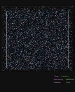
13 COGNAC Random: Amorphous like structures Helix: Helical structures at regular lattice points Crystal: Crystal structures defined by crystal data, i.e. unit lattice, symmetric operation and fractional coordinates Semi-crystalline lamella: Semi-crystalline lamella structures consisting of a crystal phase and an amorphous phase Multi phase structure: Micro/macro phase-separeted structures of block copolymer/polymer blend obtained by SUSHI
 mol")
14 mol/pdb UDF WebLab ViewerLite (TM) mol GOURMET UDF
15 UDF PDB/car/XYZ GOURMET UDF WebLab ViewerLite (TM) car
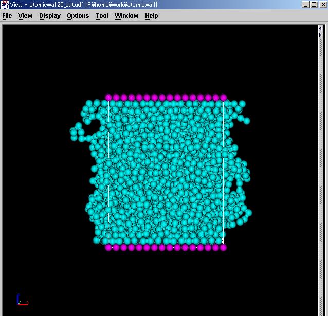
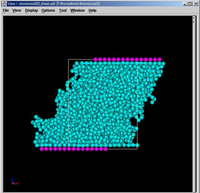
16 etc. Lees-Edwards MD»
")

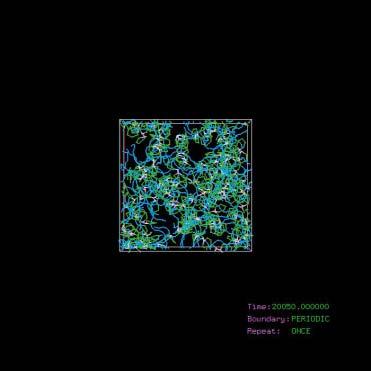
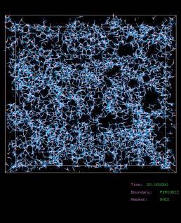
17 Clay(laponite) - Polymer(PEO) composite clay-polymer Clay
18 20nm 20nm
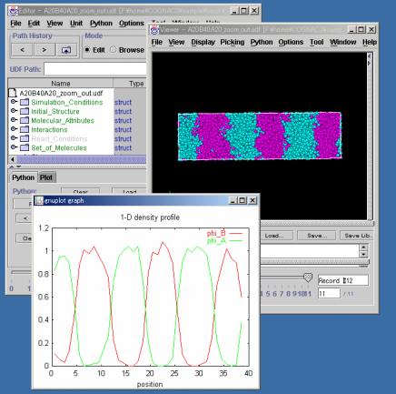
19
20 Density biased Monte Carlo (DBMC) Density biased potential (DBP) SUSHI Staggered reflective boundary condition (SRBC) Lamella builder

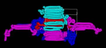
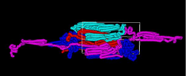
21 ABA triblock copolymer ABA triblock copolymer SUSHI Loop/Bridge


22 ABA triblock copolymer 300% Strain BCC sphere phase εσ

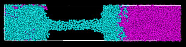
23 A/B εσ ε τ elongation δε δε δε δε
24 6nm elongation
25 COGNAC C++ COGNAC UserBond1, UserAngle1 #include "userbond1.h" double UserBond1::calcforce(const Vector3d& dr, Vector3d& ftmp) { double r,delr,ene,tmp; } r=dr.length(); delr=r-r0; tmp=kconst*delr; ftmp=dr*(tmp/r); ene=0.5*tmp*delr; return ene;
26 DPD Dissipative particle dynamics (DPD) dr dt i dv = vi, dt i = f i f i F C ij = ( C D R F + + ) ij Fij Fij i j aij = 0 ( 1 r ) ( < ) ij rˆ ij rij ( r 1) ij 1, F D ij D = w ( )( ) R R r ( ) ij rˆ ij vij rˆ ij, Fij = w rij ijrˆ ij

27 Action Python molecules/atoms/bonds ABA triblock copolymers A
28 COGNAC Python»»»»»»
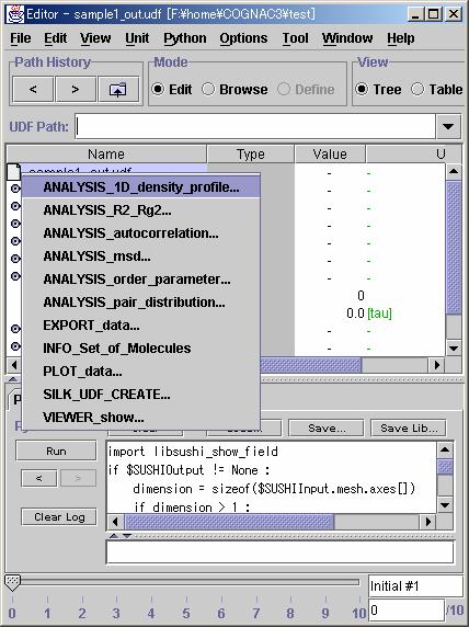
29 GOURMET Action GOURMET Action
30 :
31 : -
32 UDF HELP
![COGNAC UDF unit parameters reduced mass in [amu]](/docs-images/78/78557703/images/33-1.jpg "reduced energy in [kj/mol] reduced length in [nm].")
33 COGNAC UDF unit parameters reduced mass in [amu] reduced energy in [kj/mol] reduced length in [nm].
34 COGNAC: χ MUFFIN SUSHI PASTA COGNAC
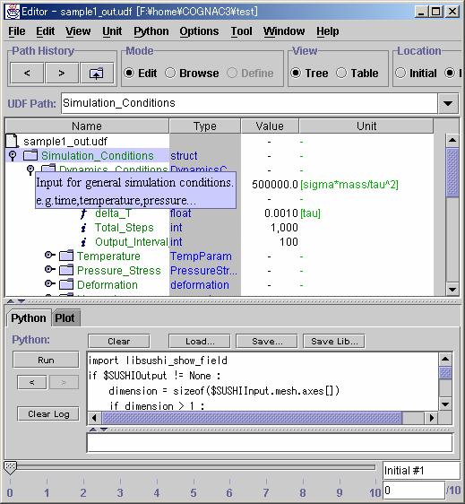
35 COGNAC : MD/MM
36 COGNAC JCII
OCTAプロジェクト:物質の多階層シミュレーション
 SS HPC 2003 2003/10/03 OCTA : www.stat.cse.nagoya-u.ac.jp,, 1 SS HPC 2003 2003/10/03 OCTA Open Computational Tool for Advanced material technology 8 2 SS HPC 2003 2003/10/03 Advanced Material Technology
MUFFIN3
 MUFFIN - MUltiFarious FIeld simulator for Non-equilibrium system - ( ) MUFFIN WG3 - - JCII, - ( ) - ( ) - ( ) - (JSR) - - MUFFIN sec -3 msec -6 sec GOURMET SUSHI MUFFIN -9 nsec PASTA -1 psec -15 fsec COGNAC
スライド タイトルなし
 J-OCTA/OCTA と LAMMPS の連携によるメリット http://www.j-octa.com/ 2016 年 2 月 19 日株式会社 JSOL エンジニアリングビジネス事業部 JSOL について 社員数 1300 人 計算科学分野は 150 人 20 以上のシミュレーション, CAE(Computer Aided Engineering) ソフトウェアミクロからマクロまで 幅広いソリューション
4/15 No.
 4/15 No. 1 4/15 No. 4/15 No. 3 Particle of mass m moving in a potential V(r) V(r) m i ψ t = m ψ(r,t)+v(r)ψ(r,t) ψ(r,t) = ϕ(r)e iωt ψ(r,t) Wave function steady state m ϕ(r)+v(r)ϕ(r) = εϕ(r) Eigenvalue problem
19 σ = P/A o σ B Maximum tensile strength σ % 0.2% proof stress σ EL Elastic limit Work hardening coefficient failure necking σ PL Proportional
 19 σ = P/A o σ B Maximum tensile strength σ 0. 0.% 0.% proof stress σ EL Elastic limit Work hardening coefficient failure necking σ PL Proportional limit ε p = 0.% ε e = σ 0. /E plastic strain ε = ε e
80 4 r ˆρ i (r, t) δ(r x i (t)) (4.1) x i (t) ρ i ˆρ i t = 0 i r 0 t(> 0) j r 0 + r < δ(r 0 x i (0))δ(r 0 + r x j (t)) > (4.2) r r 0 G i j (r, t) dr 0
 δ(r x i (t)) (4.1) x i (t) ρ i ˆρ i t = 0 i r 0 t(> 0) j r 0 + r < δ(r 0 x i (0))δ(r 0 + r x j (t)) > (4.2) r r 0 G i j (r, t) dr 0") 79 4 4.1 4.1.1 x i (t) x j (t) O O r 0 + r r r 0 x i (0) r 0 x i (0) 4.1 L. van. Hove 1954 space-time correlation function V N 4.1 ρ 0 = N/V i t 80 4 r ˆρ i (r, t) δ(r x i (t)) (4.1) x i (t) ρ i ˆρ i t
79 4 4.1 4.1.1 x i (t) x j (t) O O r 0 + r r r 0 x i (0) r 0 x i (0) 4.1 L. van. Hove 1954 space-time correlation function V N 4.1 ρ 0 = N/V i t 80 4 r ˆρ i (r, t) δ(r x i (t)) (4.1) x i (t) ρ i ˆρ i t
untitled
 SPring-8 RFgun JASRI/SPring-8 6..7 Contents.. 3.. 5. 6. 7. 8. . 3 cavity γ E A = er 3 πε γ vb r B = v E c r c A B A ( ) F = e E + v B A A A A B dp e( v B+ E) = = m d dt dt ( γ v) dv e ( ) dt v B E v E
 CMP Technical Report No. 4 Department of Computational Nanomaterials Design ISIR, Osaka University 2 2................................. 2.2......................... 2 3 3 3................................
D v D F v/d F v D F η v D (3.2) (a) F=0 (b) v=const. D F v Newtonian fluid σ ė σ = ηė (2.2) ė kl σ ij = D ijkl ė kl D ijkl (2.14) ė ij (3.3) µ η visco
 (a) F=0 (b) v=const. D F v Newtonian fluid σ ė σ = ηė (2.2) ė kl σ ij = D ijkl ė kl D ijkl (2.14) ė ij (3.3) µ η visco") post glacial rebound 3.1 Viscosity and Newtonian fluid f i = kx i σ ij e kl ideal fluid (1.9) irreversible process e ij u k strain rate tensor (3.1) v i u i / t e ij v F 23 D v D F v/d F v D F η v D (3.2)
post glacial rebound 3.1 Viscosity and Newtonian fluid f i = kx i σ ij e kl ideal fluid (1.9) irreversible process e ij u k strain rate tensor (3.1) v i u i / t e ij v F 23 D v D F v/d F v D F η v D (3.2)
株式会社ローソン 第26期中間事業報告書
 1 2 3 4 5 797 429 316 1,881 7,583 204 649 334 1,950 564 459 73.10 4,836 3,535 79.05 5,113 4,042 79.96 5,683 4,544 82.41 6,252 5,152 83.47 6,649 5,550 85.75 7,016 6,016 88.45 7,378 6,526 88.95 7,583 6,745
 1 1 1 1-1 1 1-9 1-3 1-1 13-17 -3 6-4 6 3 3-1 35 3-37 3-3 38 4 4-1 39 4- Fe C TEM 41 4-3 C TEM 44 4-4 Fe TEM 46 4-5 5 4-6 5 5 51 6 5 1 1-1 1991 1,1 multiwall nanotube 1993 singlewall nanotube ( 1,) sp 7.4eV


SAXS Table 1 DSC POM SAXSSAXS PF BL-10C BL-15A Fig. 2 LC12 DSC SAXS 138 C T iso T iso SAXS q=1.4 nm -1 q=(4π/λ)sin(θ/2), λ:, θ: Fig. 3 LC12 T iso Figu
sin(θ/2), λ:, θ: Fig. 3 LC12 T iso Figu") 1 1 1 1,2 1,2 1 2 Correlation between Microphase Separation and Liquid Crystallization in Structure Formation of Liquid Crystalline Block Copolymers Shin-ichi TANIGUCHI 1, Hiroki TAKESHITA 1, Masamitsu
1 1 1 1,2 1,2 1 2 Correlation between Microphase Separation and Liquid Crystallization in Structure Formation of Liquid Crystalline Block Copolymers Shin-ichi TANIGUCHI 1, Hiroki TAKESHITA 1, Masamitsu
Sample function Re random process Flutter, Galloping, etc. ensemble (mean value) N 1 µ = lim xk( t1) N k = 1 N autocorrelation function N 1 R( t1, t1
 N 1 µ = lim xk( t1) N k = 1 N autocorrelation function N 1 R( t1, t1") Sample function Re random process Flutter, Galloping, etc. ensemble (mean value) µ = lim xk( k = autocorrelation function R( t, t + τ) = lim ( ) ( + τ) xk t xk t k = V p o o R p o, o V S M R realization
Sample function Re random process Flutter, Galloping, etc. ensemble (mean value) µ = lim xk( k = autocorrelation function R( t, t + τ) = lim ( ) ( + τ) xk t xk t k = V p o o R p o, o V S M R realization
42 1 Fig. 2. Li 2 B 4 O 7 crystals with 3inches and 4inches in diameter. Fig. 4. Transmission curve of Li 2 B 4 O 7 crystal. Fig. 5. Refractive index
 MEMOIRS OF SHONAN INSTITUTE OF TECHNOLOGY Vol. 42, No. 1, 2008 Li 2 B 4 O 7 (LBO) *, ** * ** ** Optical Scatterer and Crystal Growth Technology of LBO Single Crystal For Development with Optical Application
i
 009 I 1 8 5 i 0 1 0.1..................................... 1 0.................................................. 1 0.3................................. 0.4........................................... 3
( ) ) AGD 2) 7) 1
 ) AGD 2) 7) 1") ( 9 5 6 ) ) AGD ) 7) S. ψ (r, t) ψ(r, t) (r, t) Ĥ ψ(r, t) = e iĥt/ħ ψ(r, )e iĥt/ħ ˆn(r, t) = ψ (r, t)ψ(r, t) () : ψ(r, t)ψ (r, t) ψ (r, t)ψ(r, t) = δ(r r ) () ψ(r, t)ψ(r, t) ψ(r, t)ψ(r, t) = (3) ψ (r,
( 9 5 6 ) ) AGD ) 7) S. ψ (r, t) ψ(r, t) (r, t) Ĥ ψ(r, t) = e iĥt/ħ ψ(r, )e iĥt/ħ ˆn(r, t) = ψ (r, t)ψ(r, t) () : ψ(r, t)ψ (r, t) ψ (r, t)ψ(r, t) = δ(r r ) () ψ(r, t)ψ(r, t) ψ(r, t)ψ(r, t) = (3) ψ (r,
BIT -2-
 2004.3.31 10 11 12-1- BIT -2- -3-256 258 932 524 585 -4- -5- A B A B AB A B A B C AB A B AB AB AB AB -6- -7- A B -8- -9- -10- mm -11- fax -12- -13- -14- -15- s58.10.1 1255 4.2 30.10-16- -17- -18- -19-6.12.10
untitled
 1 2 3 4 5 130mm 32mm UV-irradiation UV-cationic cure UV-cationic cure UV-cationic cure Thermal cationic Reaction heat cure Thermal cationic Cation Reaction heat cure Cation (a) UV-curing of
Nosé Hoover 1.2 ( 1) (a) (b) 1:
 (a) (b) 1:") 1 [email protected] 1 1.1 Nosé Hoover 1. ( 1) (a) (b) 1: T ( f(p x, p y, p z ) exp p x + p y + p ) z (1) mk B T p x p y p = = z = 1 m m m k BT () k B T = 1.3 0.04 0.03 0.0 0.01 0-5 -4-3 - -1 0
1 [email protected] 1 1.1 Nosé Hoover 1. ( 1) (a) (b) 1: T ( f(p x, p y, p z ) exp p x + p y + p ) z (1) mk B T p x p y p = = z = 1 m m m k BT () k B T = 1.3 0.04 0.03 0.0 0.01 0-5 -4-3 - -1 0
第62巻 第1号 平成24年4月/石こうを用いた木材ペレット
 Bulletin of Japan Association for Fire Science and Engineering Vol. 62. No. 1 (2012) Development of Two-Dimensional Simple Simulation Model and Evaluation of Discharge Ability for Water Discharge of Firefighting


LLG-R8.Nisus.pdf
 d M d t = γ M H + α M d M d t M γ [ 1/ ( Oe sec) ] α γ γ = gµ B h g g µ B h / π γ g = γ = 1.76 10 [ 7 1/ ( Oe sec) ] α α = λ γ λ λ λ α γ α α H α = γ H ω ω H α α H K K H K / M 1 1 > 0 α 1 M > 0 γ α γ =
ii 3.,. 4. F. (), ,,. 8.,. 1. (75%) (25%) =7 20, =7 21 (. ). 1.,, (). 3.,. 1. ().,.,.,.,.,. () (12 )., (), 0. 2., 1., 0,.
, ,,. 8.,. 1. (75%) (25%) =7 20, =7 21 (. ). 1.,, (). 3.,. 1. ().,.,.,.,.,. () (12 )., (), 0. 2., 1., 0,.") 24(2012) (1 C106) 4 11 (2 C206) 4 12 http://www.math.is.tohoku.ac.jp/~obata,.,,,.. 1. 2. 3. 4. 5. 6. 7.,,. 1., 2007 (). 2. P. G. Hoel, 1995. 3... 1... 2.,,. ii 3.,. 4. F. (),.. 5... 6.. 7.,,. 8.,. 1. (75%)
24(2012) (1 C106) 4 11 (2 C206) 4 12 http://www.math.is.tohoku.ac.jp/~obata,.,,,.. 1. 2. 3. 4. 5. 6. 7.,,. 1., 2007 (). 2. P. G. Hoel, 1995. 3... 1... 2.,,. ii 3.,. 4. F. (),.. 5... 6.. 7.,,. 8.,. 1. (75%)
positron 1930 Dirac 1933 Anderson m 22Na(hl=2.6years), 58Co(hl=71days), 64Cu(hl=12hour) 68Ge(hl=288days) MeV : thermalization m psec 100
, 58Co(hl=71days), 64Cu(hl=12hour) 68Ge(hl=288days) MeV : thermalization m psec 100") positron 1930 Dirac 1933 Anderson m 22Na(hl=2.6years), 58Co(hl=71days), 64Cu(hl=12hour) 68Ge(hl=288days) 0.5 1.5MeV : thermalization 10 100 m psec 100psec nsec E total = 2mc 2 + E e + + E e Ee+ Ee-c mc
positron 1930 Dirac 1933 Anderson m 22Na(hl=2.6years), 58Co(hl=71days), 64Cu(hl=12hour) 68Ge(hl=288days) 0.5 1.5MeV : thermalization 10 100 m psec 100psec nsec E total = 2mc 2 + E e + + E e Ee+ Ee-c mc


* 1 1 (i) (ii) Brückner-Hartree-Fock (iii) (HF, BCS, HFB) (iv) (TDHF,TDHFB) (RPA) (QRPA) (v) (vi) *
 (ii) Brückner-Hartree-Fock (iii) (HF, BCS, HFB) (iv) (TDHF,TDHFB) (RPA) (QRPA) (v) (vi) *") * 1 1 (i) (ii) Brückner-Hartree-Fock (iii) (HF, BCS, HFB) (iv) (TDHF,TDHFB) (RPA) (QRPA) (v) (vi) *1 2004 1 1 ( ) ( ) 1.1 140 MeV 1.2 ( ) ( ) 1.3 2.6 10 8 s 7.6 10 17 s? Λ 2.5 10 10 s 6 10 24 s 1.4 ( m
* 1 1 (i) (ii) Brückner-Hartree-Fock (iii) (HF, BCS, HFB) (iv) (TDHF,TDHFB) (RPA) (QRPA) (v) (vi) *1 2004 1 1 ( ) ( ) 1.1 140 MeV 1.2 ( ) ( ) 1.3 2.6 10 8 s 7.6 10 17 s? Λ 2.5 10 10 s 6 10 24 s 1.4 ( m
V(x) m e V 0 cos x π x π V(x) = x < π, x > π V 0 (i) x = 0 (V(x) V 0 (1 x 2 /2)) n n d 2 f dξ 2ξ d f 2 dξ + 2n f = 0 H n (ξ) (ii) H
 m e V 0 cos x π x π V(x) = x < π, x > π V 0 (i) x = 0 (V(x) V 0 (1 x 2 /2)) n n d 2 f dξ 2ξ d f 2 dξ + 2n f = 0 H n (ξ) (ii) H") 199 1 1 199 1 1. Vx) m e V cos x π x π Vx) = x < π, x > π V i) x = Vx) V 1 x /)) n n d f dξ ξ d f dξ + n f = H n ξ) ii) H n ξ) = 1) n expξ ) dn dξ n exp ξ )) H n ξ)h m ξ) exp ξ )dξ = π n n!δ n,m x = Vx)
199 1 1 199 1 1. Vx) m e V cos x π x π Vx) = x < π, x > π V i) x = Vx) V 1 x /)) n n d f dξ ξ d f dξ + n f = H n ξ) ii) H n ξ) = 1) n expξ ) dn dξ n exp ξ )) H n ξ)h m ξ) exp ξ )dξ = π n n!δ n,m x = Vx)
EGunGPU
 Super Computing in Accelerator simulations - Electron Gun simulation using GPGPU - K. Ohmi, KEK-Accel Accelerator Physics seminar 2009.11.19 Super computers in KEK HITACHI SR11000 POWER5 16 24GB 16 134GFlops,
96 7 1m =2 10 7 N 1A 7.1 7.2 a C (1) I (2) A C I A A a A a A A a C C C 7.2: C A C A = = µ 0 2π (1) A C 7.2 AC C A 3 3 µ0 I 2 = 2πa. (2) A C C 7.2 A A
 I (2) A C I A A a A a A A a C C C 7.2: C A C A = = µ 0 2π (1) A C 7.2 AC C A 3 3 µ0 I 2 = 2πa. (2) A C C 7.2 A A") 7 Lorentz 7.1 Ampère I 1 I 2 I 2 I 1 L I 1 I 2 21 12 L r 21 = 12 = µ 0 2π I 1 I 2 r L. (7.1) 7.1 µ 0 =4π 10 7 N A 2 (7.2) magnetic permiability I 1 I 2 I 1 I 2 12 21 12 21 7.1: 1m 95 96 7 1m =2 10 7 N
7 Lorentz 7.1 Ampère I 1 I 2 I 2 I 1 L I 1 I 2 21 12 L r 21 = 12 = µ 0 2π I 1 I 2 r L. (7.1) 7.1 µ 0 =4π 10 7 N A 2 (7.2) magnetic permiability I 1 I 2 I 1 I 2 12 21 12 21 7.1: 1m 95 96 7 1m =2 10 7 N

42 3 u = (37) MeV/c 2 (3.4) [1] u amu m p m n [1] m H [2] m p = (4) MeV/c 2 = (13) u m n = (4) MeV/c 2 =
![42 3 u = (37) MeV/c 2 (3.4) [1] u amu m p m n [1] m H [2] m p = (4) MeV/c 2 = (13) u m n = (4) MeV/c 2 =](/thumbs/73/68712188.jpg "42 3 u = (37) MeV/c 2 (3.4) [1] u amu m p m n [1] m H [2] m p = (4) MeV/c 2 = (13) u m n = (4) MeV/c 2 =") 3 3.1 3.1.1 kg m s J = kg m 2 s 2 MeV MeV [1] 1MeV=1 6 ev = 1.62 176 462 (63) 1 13 J (3.1) [1] 1MeV/c 2 =1.782 661 731 (7) 1 3 kg (3.2) c =1 MeV (atomic mass unit) 12 C u = 1 12 M(12 C) (3.3) 41 42 3 u
3 3.1 3.1.1 kg m s J = kg m 2 s 2 MeV MeV [1] 1MeV=1 6 ev = 1.62 176 462 (63) 1 13 J (3.1) [1] 1MeV/c 2 =1.782 661 731 (7) 1 3 kg (3.2) c =1 MeV (atomic mass unit) 12 C u = 1 12 M(12 C) (3.3) 41 42 3 u
2 Chapter 4 (f4a). 2. (f4cone) ( θ) () g M. 2. (f4b) T M L P a θ (f4eki) ρ H A a g. v ( ) 2. H(t) ( )
. 2. (f4cone) ( θ) () g M. 2. (f4b) T M L P a θ (f4eki) ρ H A a g. v ( ) 2. H(t) ( )") http://astr-www.kj.yamagata-u.ac.jp/~shibata f4a f4b 2 f4cone f4eki f4end 4 f5meanfp f6coin () f6a f7a f7b f7d f8a f8b f9a f9b f9c f9kep f0a f0bt version feqmo fvec4 fvec fvec6 fvec2 fvec3 f3a (-D) f3b
http://astr-www.kj.yamagata-u.ac.jp/~shibata f4a f4b 2 f4cone f4eki f4end 4 f5meanfp f6coin () f6a f7a f7b f7d f8a f8b f9a f9b f9c f9kep f0a f0bt version feqmo fvec4 fvec fvec6 fvec2 fvec3 f3a (-D) f3b
1
 GL (a) (b) Ph l P N P h l l Ph Ph Ph Ph l l l l P Ph l P N h l P l .9 αl B βlt D E. 5.5 L r..8 e g s e,e l l W l s l g W W s g l l W W e s g e s g r e l ( s ) l ( l s ) r e l ( s ) l ( l s ) e R e r
JFE.dvi
 ,, Department of Civil Engineering, Chuo University Kasuga 1-13-27, Bunkyo-ku, Tokyo 112 8551, JAPAN E-mail : [email protected] E-mail : [email protected] SATO KOGYO CO., LTD. 12-20, Nihonbashi-Honcho
5 H Boltzmann Einstein Brown 5.1 Onsager [ ] Tr Tr Tr = dγ (5.1) A(p, q) Â 0 = Tr Âe βĥ0 Tr e βĥ0 = dγ e βh 0(p,q) A(p, q) dγ e βh 0(p,q) (5.2) e βĥ0
![5 H Boltzmann Einstein Brown 5.1 Onsager [ ] Tr Tr Tr = dγ (5.1) A(p, q) Â 0 = Tr Âe βĥ0 Tr e βĥ0 = dγ e βh 0(p,q) A(p, q) dγ e βh 0(p,q) (5.2) e βĥ0](/thumbs/99/141438380.jpg "5 H Boltzmann Einstein Brown 5.1 Onsager [ ] Tr Tr Tr = dγ (5.1) A(p, q) Â 0 = Tr Âe βĥ0 Tr e βĥ0 = dγ e βh 0(p,q) A(p, q) dγ e βh 0(p,q) (5.2) e βĥ0") 5 H Boltzmann Einstein Brown 5.1 Onsager [ ] Tr Tr Tr = dγ (5.1) A(p, q) Â = Tr Âe βĥ Tr e βĥ = dγ e βh (p,q) A(p, q) dγ e βh (p,q) (5.2) e βĥ A(p, q) p q Â(t) = Tr Â(t)e βĥ Tr e βĥ = dγ() e βĥ(p(),q())
5 H Boltzmann Einstein Brown 5.1 Onsager [ ] Tr Tr Tr = dγ (5.1) A(p, q) Â = Tr Âe βĥ Tr e βĥ = dγ e βh (p,q) A(p, q) dγ e βh (p,q) (5.2) e βĥ A(p, q) p q Â(t) = Tr Â(t)e βĥ Tr e βĥ = dγ() e βĥ(p(),q())
 1-1 (1) (3) 16.6 6.6 60.9 82.2 32.1 1980 199 1-2 1-3 (2) (2001) 2001 2-1 P A e U ij A ij = e Uij R + e U ij A + e U ij C U ija = a 0 +a 1 c ija +a 2 T ija +a 3 AT ija + Air i Rail Car
t χ 2 F Q t χ 2 F 1 2 µ, σ 2 N(µ, σ 2 ) f(x µ, σ 2 ) = 1 ( exp (x ) µ)2 2πσ 2 2σ 2 0, N(0, 1) (100 α) z(α) t χ 2 *1 2.1 t (i)x N(µ, σ 2 ) x µ σ N(0, 1
 f(x µ, σ 2 ) = 1 ( exp (x ) µ)2 2πσ 2 2σ 2 0, N(0, 1) (100 α) z(α) t χ 2 *1 2.1 t (i)x N(µ, σ 2 ) x µ σ N(0, 1") t χ F Q t χ F µ, σ N(µ, σ ) f(x µ, σ ) = ( exp (x ) µ) πσ σ 0, N(0, ) (00 α) z(α) t χ *. t (i)x N(µ, σ ) x µ σ N(0, ) (ii)x,, x N(µ, σ ) x = x+ +x N(µ, σ ) (iii) (i),(ii) z = x µ N(0, ) σ N(0, ) ( 9 97.
t χ F Q t χ F µ, σ N(µ, σ ) f(x µ, σ ) = ( exp (x ) µ) πσ σ 0, N(0, ) (00 α) z(α) t χ *. t (i)x N(µ, σ ) x µ σ N(0, ) (ii)x,, x N(µ, σ ) x = x+ +x N(µ, σ ) (iii) (i),(ii) z = x µ N(0, ) σ N(0, ) ( 9 97.
δ ij δ ij ˆx ˆx ŷ ŷ ẑ ẑ 0, ˆx ŷ ŷ ˆx ẑ, ŷ ẑ ẑ ŷ ẑ, ẑ ˆx ˆx ẑ ŷ, a b a x ˆx + a y ŷ + a z ẑ b x ˆx + b
 23 2 2.1 n n r x, y, z ˆx ŷ ẑ 1 a a x ˆx + a y ŷ + a z ẑ 2.1.1 3 a iˆx i. 2.1.2 i1 i j k e x e y e z 3 a b a i b i i 1, 2, 3 x y z ˆx i ˆx j δ ij, 2.1.3 n a b a i b i a i b i a x b x + a y b y + a z b
The Evaluation on Impact Strength of Structural Elements by Means of Drop Weight Test Elastic Response and Elastic Limit by Hiroshi Maenaka, Member Sh
 The Evaluation on Impact Strength of Structural Elements by Means of Drop Weight Test Elastic Response and Elastic Limit by Hiroshi Maenaka, Member Shigeru Kitamura, Member Masaaki Sakuma Genya Aoki, Member
