MUFFIN3
|
|
|
- うたろう おいもり
- 8 years ago
- Views:
Transcription
1 MUFFIN - MUltiFarious FIeld simulator for Non-equilibrium system - ( )
2 MUFFIN WG3 - - JCII, - ( ) - ( ) - ( ) - (JSR) - -
3 MUFFIN sec -3 msec -6 sec GOURMET SUSHI MUFFIN -9 nsec PASTA -1 psec -15 fsec COGNAC fm pm nm m mm m
4 MUFFIN
5 MUFFIN - (FDM) : - (FEM) :. - - (D/3D). ( D/3D) or - : -,,,,. - : Navier-Stokes, Stokes, Oseen,,.. - :,. - :, -,
6 MUFFIN SuperField. ( ) - DynamicsManager. - MUFFIN SuperField B.C. Dynamics Manager UDF(XML) MUFFIN API ( ) - MUFFIN -
 Prof.")

7 MUFFIN - - cf) XSIL (XML Scientific Interchange) Prof. R.Williams, CACR, Caltech. (Center for Advanced Computing Research)


8 MUFFIN ( ) PhaseSeparation Electrolyte MEMFluid Elastica GelDyna TURBAN shear PhaseSeparation : GelDyna : TURBAN : Elastica : Electrolyte MEMFluid :
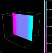
9 PhaseSeparation : ψ t v ρ t v α = = = ( ψ p α + v ) + ( L α µ α [ { v + ( v) }] t η ) + K, Stokes flow / t =, K. L
10 =
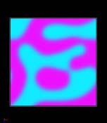
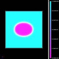
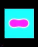
11 PhaseSeparation FDM t=1 t=4 t= Flory-Huggins t= t= t=1
12 PhaseSeparation FDM

 Macromolecules,")
")
13 ( PhaseSeparation FDM ) Macromolecules, 9, 33 (1996) Macromolecules, 3, 4995 (1997) Macromolecules, 3, 4995 (1997) Macromolecules, 9, 33 (1996) Polymer, 4, 111 (1)

 = κ 1 κ x 1 x")
14 J. Electrochem. Soc., 138, 317 (1991) E ( x 1 x ) = κ 1 κ x 1 x 1
 - PMMA /")

 (E")
15 (csolv-poly) - Poly1 / Poly / solvent (Poly1 ) - PMMA / PS / MEK (PMMA ) (gs ) - Poly1 / Poly /substrate (better for Poly) - PMMA / PS / ODM (better for PS) (E ) - (h ) -
16 Electrolyte 3 FDM FEM Electrolyte
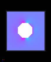
17 Electrolyte FDM t=1 t=1 t=1 t=1 ( )
18 Electrolyte FEM
 E E")
19 Electrolyte FEM : ( ) E E E E
![MEMFluid Cα : Cα ( ) = ( vcα ) jα + R1αβ Cβ + Rαβγ CβC t : jα = Lα [ kbt{ Cα + χαβcα Cβ } + ezαcα ( Φ E)] Oseen ( Laplace : [ { v ( v) }] t ) = p + η w + + K } : K = k B T{ Cα + χ](/docs-images/78/78557690/images/20-0.jpg "αβcα Cβ } α β : Φ = β β β, γ ( v = ) ( ) : j α : L α : Z α : χ αβ : Φ : E : MEMS (Micro Electro Mechanical System), Lab-on-a chip.")
20 MEMFluid Cα : Cα ( ) = ( vcα ) jα + R1αβ Cβ + Rαβγ CβC t : jα = Lα [ kbt{ Cα + χαβcα Cβ } + ezαcα ( Φ E)] Oseen ( Laplace : [ { v ( v) }] t ) = p + η w + + K } : K = k B T{ Cα + χ αβcα Cβ } α β : Φ = β β β, γ ( v = ) ( ) : j α : L α : Z α : χ αβ : Φ : E : MEMS (Micro Electro Mechanical System), Lab-on-a chip. Micro reactor, TAS (Total Analysis System), Bio chips. γ


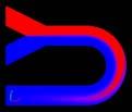
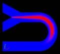
21 MEMFluid Y A C 4sec 6sec 8sec 1sec 16cases: Productivity (Pc) of C-ion P=1.,.5,5.,1. vs logr and log P R=1e-3,1e-,1e-1,1. Results: For increase Pc. R >.4: P->1. R <.4: P->1.
 ς = k T σ ln[ (8Cεk T ) σ ( 8Cεk B 1 / + + 1) 1 / Ze B BT - ( ) Ze ς / kbt << 1 ς 5( mv ) { σ ς = εκ ZαCα e α 1 / κ = ( ) εk")
22 MEMFluid : ε veo = ςe Helmholtz-Smouluchowski eq. ηw -potential : -1 Poisson-Boltzmann eq. (1-1 electrolyte) ς = k T σ ln[ (8Cεk T ) σ ( 8Cεk B 1 / + + 1) 1 / Ze B BT - ( ) Ze ς / kbt << 1 ς 5( mv ) { σ ς = εκ ZαCα e α 1 / κ = ( ) εk T B : / : l b l = e ( k B 1 Tεl) 3 1 ] : P=1., R=1.
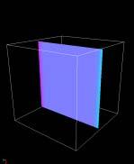
23 Elastica, 3 FEM F d { u ( x) } = d x{ f } i V f V d 1 = G x ) e δ e + ij ij ll d d xρ( x) g u ( x) i K( x) i ( e ) ( ll e ij = 1 ui x j u + x St d d 1 xt i u i ( x) ( e ) ( ) ii + D nin jeij + D 3(ell nin jeij ) + D4nleil nkeik D eijeij f = D1 + 5 j j
24 + + = xy zx yz zz yy xx xy zx yz zz yy xx e e e e e e m m k m k l m k m k l l l n µ µ σ σ σ σ σ σ ( ) ( ) ij ij ik k il l ij j i ll ij j i ii e D e e n D n e ) e n n D (e e n n D e D f = ( ) ( ) = = + = + = = m D m D m k l D l m k n D m k D µ µ


25 Elastica : SUSHI : 1( ) z, x,y x,y, z :

26 Elastica :.µm 1.µm

27 Elastica : Morphology (PP + Elastomer) F = G e ij 1 δ ije d ll + K 1 e kk (a)dispersed (b)bi-continuous (C) by SUSHI Young K = e ij 1 δ ije d 1 e kk ll G + F 1 e kk modulus E analytic-model sphere series bi-continuous Davies sushi sushi 5.99 sushi: volume fraction is reset to and 1 using a threshold value.
28 GelDyna : ς ( v p v s ) = φ p + : ς ( v s v p ) = ( 1 φ ) : [ φ v + ( 1 φ ) v ] = p s p σ ( ) v p : v s : φ : p : ς : σ : k BT d 1 φ = d x[(1 φ ) ln( 1 φ ) + χφ (1 φ ) + ν ( tr v φ F W + φ σ ij = [ φ f m ' ( φ ) f m ( φ )] δ ij + ν ( W ij δ ij ) φ (Flory-Huggins): ( φ ) = (1 φ ) ln( 1 φ ) + χφ (1 φ ) W ij : φ : χ : : ν f m ln 1 φ φ )]
")


29 GelDyna (DDS) NIPA D 3D

 (ii)")
30 TURBAN =TURBidity ANalyzer TURBAN TURBAN : (i) (ii) Maxwell
31 : = 4-7nm - -PE : TURBAN PE


32 MUFFIN MILK ( ) - 3D/D - - NASTRAN BULK FILTER - NASTRAN BULK UDF. HyperMesh UDF GOURMET MeshFieldConvertor (IMPORT/EXPORT_...) -SUSHI
 - UDF AVS - - - (gnuplot ).")
33 udfavs MUFFIN MeshFieldShow (SHOW_...) - - MeshFieldPlot (PLOT_...) - UDF AVS (gnuplot ) ModelingSupporter, analyze_reactor,
34 MUFFIN : SUSHI MUFFIN PASTA COGNAC
35 MUFFIN (MUltiFarious FIeld simulator for Non-equilibrium system) (.1 m 1mm, sec) PhaseSeparation, Electrolyte, MEMFluid, Elastica, GelDyna, TURBAN MUFFIN MUFFIN
OCTAプロジェクト:物質の多階層シミュレーション
 SS HPC 2003 2003/10/03 OCTA : www.stat.cse.nagoya-u.ac.jp,, 1 SS HPC 2003 2003/10/03 OCTA Open Computational Tool for Advanced material technology 8 2 SS HPC 2003 2003/10/03 Advanced Material Technology
n (1.6) i j=1 1 n a ij x j = b i (1.7) (1.7) (1.4) (1.5) (1.4) (1.7) u, v, w ε x, ε y, ε x, γ yz, γ zx, γ xy (1.8) ε x = u x ε y = v y ε z = w z γ yz
 i j=1 1 n a ij x j = b i (1.7) (1.7) (1.4) (1.5) (1.4) (1.7) u, v, w ε x, ε y, ε x, γ yz, γ zx, γ xy (1.8) ε x = u x ε y = v y ε z = w z γ yz") 1 2 (a 1, a 2, a n ) (b 1, b 2, b n ) A (1.1) A = a 1 b 1 + a 2 b 2 + + a n b n (1.1) n A = a i b i (1.2) i=1 n i 1 n i=1 a i b i n i=1 A = a i b i (1.3) (1.3) (1.3) (1.1) (ummation convention) a 11 x
1 2 (a 1, a 2, a n ) (b 1, b 2, b n ) A (1.1) A = a 1 b 1 + a 2 b 2 + + a n b n (1.1) n A = a i b i (1.2) i=1 n i 1 n i=1 a i b i n i=1 A = a i b i (1.3) (1.3) (1.3) (1.1) (ummation convention) a 11 x
No δs δs = r + δr r = δr (3) δs δs = r r = δr + u(r + δr, t) u(r, t) (4) δr = (δx, δy, δz) u i (r + δr, t) u i (r, t) = u i x j δx j (5) δs 2
 δs δs = r r = δr + u(r + δr, t) u(r, t) (4) δr = (δx, δy, δz) u i (r + δr, t) u i (r, t) = u i x j δx j (5) δs 2") No.2 1 2 2 δs δs = r + δr r = δr (3) δs δs = r r = δr + u(r + δr, t) u(r, t) (4) δr = (δx, δy, δz) u i (r + δr, t) u i (r, t) = u i δx j (5) δs 2 = δx i δx i + 2 u i δx i δx j = δs 2 + 2s ij δx i δx j
No.2 1 2 2 δs δs = r + δr r = δr (3) δs δs = r r = δr + u(r + δr, t) u(r, t) (4) δr = (δx, δy, δz) u i (r + δr, t) u i (r, t) = u i δx j (5) δs 2 = δx i δx i + 2 u i δx i δx j = δs 2 + 2s ij δx i δx j
k m m d2 x i dt 2 = f i = kx i (i = 1, 2, 3 or x, y, z) f i σ ij x i e ij = 2.1 Hooke s law and elastic constants (a) x i (2.1) k m σ A σ σ σ σ f i x
 f i σ ij x i e ij = 2.1 Hooke s law and elastic constants (a) x i (2.1) k m σ A σ σ σ σ f i x") k m m d2 x i dt 2 = f i = kx i (i = 1, 2, 3 or x, y, z) f i ij x i e ij = 2.1 Hooke s law and elastic constants (a) x i (2.1) k m A f i x i B e e e e 0 e* e e (2.1) e (b) A e = 0 B = 0 (c) (2.1) (d) e
k m m d2 x i dt 2 = f i = kx i (i = 1, 2, 3 or x, y, z) f i ij x i e ij = 2.1 Hooke s law and elastic constants (a) x i (2.1) k m A f i x i B e e e e 0 e* e e (2.1) e (b) A e = 0 B = 0 (c) (2.1) (d) e
第86回日本感染症学会総会学術集会後抄録(I)
") κ κ κ κ κ κ μ μ β β β γ α α β β γ α β α α α γ α β β γ μ β β μ μ α ββ β β β β β β β β β β β β β β β β β β γ β μ μ μ μμ μ μ μ μ β β μ μ μ μ μ μ μ μ μ μ μ μ μ μ β
κ κ κ κ κ κ μ μ β β β γ α α β β γ α β α α α γ α β β γ μ β β μ μ α ββ β β β β β β β β β β β β β β β β β β γ β μ μ μ μμ μ μ μ μ β β μ μ μ μ μ μ μ μ μ μ μ μ μ μ β
変 位 変位とは 物体中のある点が変形後に 別の点に異動したときの位置の変化で あり ベクトル量である 変位には 物体の変形の他に剛体運動 剛体変位 が含まれている 剛体変位 P(x, y, z) 平行移動と回転 P! (x + u, y + v, z + w) Q(x + d x, y + dy,
 平行移動と回転 P! (x + u, y + v, z + w) Q(x + d x, y + dy,") 変 位 変位とは 物体中のある点が変形後に 別の点に異動したときの位置の変化で あり ベクトル量である 変位には 物体の変形の他に剛体運動 剛体変位 が含まれている 剛体変位 P(x, y, z) 平行移動と回転 P! (x + u, y + v, z + w) Q(x + d x, y + dy, z + dz) Q! (x + d x + u + du, y + dy + v + dv, z +
変 位 変位とは 物体中のある点が変形後に 別の点に異動したときの位置の変化で あり ベクトル量である 変位には 物体の変形の他に剛体運動 剛体変位 が含まれている 剛体変位 P(x, y, z) 平行移動と回転 P! (x + u, y + v, z + w) Q(x + d x, y + dy, z + dz) Q! (x + d x + u + du, y + dy + v + dv, z +
all.dvi
 72 9 Hooke,,,. Hooke. 9.1 Hooke 1 Hooke. 1, 1 Hooke. σ, ε, Young. σ ε (9.1), Young. τ γ G τ Gγ (9.2) X 1, X 2. Poisson, Poisson ν. ν ε 22 (9.) ε 11 F F X 2 X 1 9.1: Poisson 9.1. Hooke 7 Young Poisson G
医系の統計入門第 2 版 サンプルページ この本の定価 判型などは, 以下の URL からご覧いただけます. このサンプルページの内容は, 第 2 版 1 刷発行時のものです.
 医系の統計入門第 2 版 サンプルページ この本の定価 判型などは, 以下の URL からご覧いただけます. http://www.morikita.co.jp/books/mid/009192 このサンプルページの内容は, 第 2 版 1 刷発行時のものです. i 2 t 1. 2. 3 2 3. 6 4. 7 5. n 2 ν 6. 2 7. 2003 ii 2 2013 10 iii 1987
 006 11 8 0 3 1 5 1.1..................... 5 1......................... 6 1.3.................... 6 1.4.................. 8 1.5................... 8 1.6................... 10 1.6.1......................
. ev=,604k m 3 Debye ɛ 0 kt e λ D = n e n e Ze 4 ln Λ ν ei = 5.6π / ɛ 0 m/ e kt e /3 ν ei v e H + +e H ev Saha x x = 3/ πme kt g i g e n
 003...............................3 Debye................. 3.4................ 3 3 3 3. Larmor Cyclotron... 3 3................ 4 3.3.......... 4 3.3............ 4 3.3...... 4 3.3.3............ 5 3.4.........
I ( ) 1 de Broglie 1 (de Broglie) p λ k h Planck ( Js) p = h λ = k (1) h 2π : Dirac k B Boltzmann ( J/K) T U = 3 2 k BT
 1 de Broglie 1 (de Broglie) p λ k h Planck ( Js) p = h λ = k (1) h 2π : Dirac k B Boltzmann ( J/K) T U = 3 2 k BT") I (008 4 0 de Broglie (de Broglie p λ k h Planck ( 6.63 0 34 Js p = h λ = k ( h π : Dirac k B Boltzmann (.38 0 3 J/K T U = 3 k BT ( = λ m k B T h m = 0.067m 0 m 0 = 9. 0 3 kg GaAs( a T = 300 K 3 fg 07345
I (008 4 0 de Broglie (de Broglie p λ k h Planck ( 6.63 0 34 Js p = h λ = k ( h π : Dirac k B Boltzmann (.38 0 3 J/K T U = 3 k BT ( = λ m k B T h m = 0.067m 0 m 0 = 9. 0 3 kg GaAs( a T = 300 K 3 fg 07345
meiji_resume_1.PDF
 β β β (q 1,q,..., q n ; p 1, p,..., p n ) H(q 1,q,..., q n ; p 1, p,..., p n ) Hψ = εψ ε k = k +1/ ε k = k(k 1) (x, y, z; p x, p y, p z ) (r; p r ), (θ; p θ ), (ϕ; p ϕ ) ε k = 1/ k p i dq i E total = E
nsg02-13/ky045059301600033210
 φ φ φ φ κ κ α α μ μ α α μ χ et al Neurosci. Res. Trpv J Physiol μ μ α α α β in vivo β β β β β β β β in vitro β γ μ δ μδ δ δ α θ α θ α In Biomechanics at Micro- and Nanoscale Levels, Volume I W W v W
液晶の物理1:連続体理論(弾性,粘性)
") The Physics of Liquid Crystals P. G. de Gennes and J. Prost (Oxford University Press, 1993) Liquid crystals are beautiful and mysterious; I am fond of them for both reasons. My hope is that some readers
The Physics of Liquid Crystals P. G. de Gennes and J. Prost (Oxford University Press, 1993) Liquid crystals are beautiful and mysterious; I am fond of them for both reasons. My hope is that some readers

I II
 I II I I 8 I I 5 I 5 9 I 6 6 I 7 7 I 8 87 I 9 96 I 7 I 8 I 9 I 7 I 95 I 5 I 6 II 7 6 II 8 II 9 59 II 67 II 76 II II 9 II 8 II 5 8 II 6 58 II 7 6 II 8 8 I.., < b, b, c, k, m. k + m + c + c b + k + m log
微分積分 サンプルページ この本の定価 判型などは, 以下の URL からご覧いただけます. このサンプルページの内容は, 初版 1 刷発行時のものです.
 微分積分 サンプルページ この本の定価 判型などは, 以下の URL からご覧いただけます. ttp://www.morikita.co.jp/books/mid/00571 このサンプルページの内容は, 初版 1 刷発行時のものです. i ii 014 10 iii [note] 1 3 iv 4 5 3 6 4 x 0 sin x x 1 5 6 z = f(x, y) 1 y = f(x)
COGNACのコンセプト \(COarse Grained molecular dynamics program developed by NAgoya Cooperation\)
") COGNAC (COarse-Grained molecular dynamics program by NAgoya Cooperation) ( ), 0 sec -3 msec -6 sec -9 nsec -12 psec -15 fsec GOURMET SUSHI PASTA COGNAC MUFFIN -15-12 -9-6 -3 0 fm pm nm m mm m United atom
COGNAC (COarse-Grained molecular dynamics program by NAgoya Cooperation) ( ), 0 sec -3 msec -6 sec -9 nsec -12 psec -15 fsec GOURMET SUSHI PASTA COGNAC MUFFIN -15-12 -9-6 -3 0 fm pm nm m mm m United atom
 21 2 26 i 1 1 1.1............................ 1 1.2............................ 3 2 9 2.1................... 9 2.2.......... 9 2.3................... 11 2.4....................... 12 3 15 3.1..........
")
4. ϵ(ν, T ) = c 4 u(ν, T ) ϵ(ν, T ) T ν π4 Planck dx = 0 e x 1 15 U(T ) x 3 U(T ) = σt 4 Stefan-Boltzmann σ 2π5 k 4 15c 2 h 3 = W m 2 K 4 5.
 = c 4 u(ν, T ) ϵ(ν, T ) T ν π4 Planck dx = 0 e x 1 15 U(T ) x 3 U(T ) = σt 4 Stefan-Boltzmann σ 2π5 k 4 15c 2 h 3 = W m 2 K 4 5.") A 1. Boltzmann Planck u(ν, T )dν = 8πh ν 3 c 3 kt 1 dν h 6.63 10 34 J s Planck k 1.38 10 23 J K 1 Boltzmann u(ν, T ) T ν e hν c = 3 10 8 m s 1 2. Planck λ = c/ν Rayleigh-Jeans u(ν, T )dν = 8πν2 kt dν c
A 1. Boltzmann Planck u(ν, T )dν = 8πh ν 3 c 3 kt 1 dν h 6.63 10 34 J s Planck k 1.38 10 23 J K 1 Boltzmann u(ν, T ) T ν e hν c = 3 10 8 m s 1 2. Planck λ = c/ν Rayleigh-Jeans u(ν, T )dν = 8πν2 kt dν c
II ( ) (7/31) II ( [ (3.4)] Navier Stokes [ (6/29)] Navier Stokes 3 [ (6/19)] Re
![II ( ) (7/31) II ( [ (3.4)] Navier Stokes [ (6/29)] Navier Stokes 3 [ (6/19)] Re](/thumbs/94/118770263.jpg "II ( ) (7/31) II ( [ (3.4)] Navier Stokes [ (6/29)] Navier Stokes 3 [ (6/19)] Re") II 29 7 29-7-27 ( ) (7/31) II (http://www.damp.tottori-u.ac.jp/~ooshida/edu/fluid/) [ (3.4)] Navier Stokes [ (6/29)] Navier Stokes 3 [ (6/19)] Reynolds [ (4.6), (45.8)] [ p.186] Navier Stokes I Euler Navier
II 29 7 29-7-27 ( ) (7/31) II (http://www.damp.tottori-u.ac.jp/~ooshida/edu/fluid/) [ (3.4)] Navier Stokes [ (6/29)] Navier Stokes 3 [ (6/19)] Reynolds [ (4.6), (45.8)] [ p.186] Navier Stokes I Euler Navier

")
V(x) m e V 0 cos x π x π V(x) = x < π, x > π V 0 (i) x = 0 (V(x) V 0 (1 x 2 /2)) n n d 2 f dξ 2ξ d f 2 dξ + 2n f = 0 H n (ξ) (ii) H
 m e V 0 cos x π x π V(x) = x < π, x > π V 0 (i) x = 0 (V(x) V 0 (1 x 2 /2)) n n d 2 f dξ 2ξ d f 2 dξ + 2n f = 0 H n (ξ) (ii) H") 199 1 1 199 1 1. Vx) m e V cos x π x π Vx) = x < π, x > π V i) x = Vx) V 1 x /)) n n d f dξ ξ d f dξ + n f = H n ξ) ii) H n ξ) = 1) n expξ ) dn dξ n exp ξ )) H n ξ)h m ξ) exp ξ )dξ = π n n!δ n,m x = Vx)
199 1 1 199 1 1. Vx) m e V cos x π x π Vx) = x < π, x > π V i) x = Vx) V 1 x /)) n n d f dξ ξ d f dξ + n f = H n ξ) ii) H n ξ) = 1) n expξ ) dn dξ n exp ξ )) H n ξ)h m ξ) exp ξ )dξ = π n n!δ n,m x = Vx)
I-2 (100 ) (1) y(x) y dy dx y d2 y dx 2 (a) y + 2y 3y = 9e 2x (b) x 2 y 6y = 5x 4 (2) Bernoulli B n (n = 0, 1, 2,...) x e x 1 = n=0 B 0 B 1 B 2 (3) co
 (1) y(x) y dy dx y d2 y dx 2 (a) y + 2y 3y = 9e 2x (b) x 2 y 6y = 5x 4 (2) Bernoulli B n (n = 0, 1, 2,...) x e x 1 = n=0 B 0 B 1 B 2 (3) co") 16 I ( ) (1) I-1 I-2 I-3 (2) I-1 ( ) (100 ) 2l x x = 0 y t y(x, t) y(±l, t) = 0 m T g y(x, t) l y(x, t) c = 2 y(x, t) c 2 2 y(x, t) = g (A) t 2 x 2 T/m (1) y 0 (x) y 0 (x) = g c 2 (l2 x 2 ) (B) (2) (1)
16 I ( ) (1) I-1 I-2 I-3 (2) I-1 ( ) (100 ) 2l x x = 0 y t y(x, t) y(±l, t) = 0 m T g y(x, t) l y(x, t) c = 2 y(x, t) c 2 2 y(x, t) = g (A) t 2 x 2 T/m (1) y 0 (x) y 0 (x) = g c 2 (l2 x 2 ) (B) (2) (1)
TOP URL 1
 TOP URL http://amonphys.web.fc.com/ 3.............................. 3.............................. 4.3 4................... 5.4........................ 6.5........................ 8.6...........................7
D v D F v/d F v D F η v D (3.2) (a) F=0 (b) v=const. D F v Newtonian fluid σ ė σ = ηė (2.2) ė kl σ ij = D ijkl ė kl D ijkl (2.14) ė ij (3.3) µ η visco
 (a) F=0 (b) v=const. D F v Newtonian fluid σ ė σ = ηė (2.2) ė kl σ ij = D ijkl ė kl D ijkl (2.14) ė ij (3.3) µ η visco") post glacial rebound 3.1 Viscosity and Newtonian fluid f i = kx i σ ij e kl ideal fluid (1.9) irreversible process e ij u k strain rate tensor (3.1) v i u i / t e ij v F 23 D v D F v/d F v D F η v D (3.2)
post glacial rebound 3.1 Viscosity and Newtonian fluid f i = kx i σ ij e kl ideal fluid (1.9) irreversible process e ij u k strain rate tensor (3.1) v i u i / t e ij v F 23 D v D F v/d F v D F η v D (3.2)
,. Black-Scholes u t t, x c u 0 t, x x u t t, x c u t, x x u t t, x + σ x u t, x + rx ut, x rux, t 0 x x,,.,. Step 3, 7,,, Step 6., Step 4,. Step 5,,.
 9 α ν β Ξ ξ Γ γ o δ Π π ε ρ ζ Σ σ η τ Θ θ Υ υ ι Φ φ κ χ Λ λ Ψ ψ µ Ω ω Def, Prop, Th, Lem, Note, Remark, Ex,, Proof, R, N, Q, C [a, b {x R : a x b} : a, b {x R : a < x < b} : [a, b {x R : a x < b} : a,
II No.01 [n/2] [1]H n (x) H n (x) = ( 1) r n! r!(n 2r)! (2x)n 2r. r=0 [2]H n (x) n,, H n ( x) = ( 1) n H n (x). [3] H n (x) = ( 1) n dn x2 e dx n e x2
![II No.01 [n/2] [1]H n (x) H n (x) = ( 1) r n! r!(n 2r)! (2x)n 2r. r=0 [2]H n (x) n,, H n ( x) = ( 1) n H n (x). [3] H n (x) = ( 1) n dn x2 e dx n e x2](/thumbs/101/149159646.jpg "II No.01 [n/2] [1]H n (x) H n (x) = ( 1) r n! r!(n 2r)! (2x)n 2r. r=0 [2]H n (x) n,, H n ( x) = ( 1) n H n (x). [3] H n (x) = ( 1) n dn x2 e dx n e x2") II No.1 [n/] [1]H n x) H n x) = 1) r n! r!n r)! x)n r r= []H n x) n,, H n x) = 1) n H n x) [3] H n x) = 1) n dn x e dx n e x [4] H n+1 x) = xh n x) nh n 1 x) ) d dx x H n x) = H n+1 x) d dx H nx) = nh
II No.1 [n/] [1]H n x) H n x) = 1) r n! r!n r)! x)n r r= []H n x) n,, H n x) = 1) n H n x) [3] H n x) = 1) n dn x e dx n e x [4] H n+1 x) = xh n x) nh n 1 x) ) d dx x H n x) = H n+1 x) d dx H nx) = nh
I A A441 : April 15, 2013 Version : 1.1 I Kawahira, Tomoki TA (Shigehiro, Yoshida )
") I013 00-1 : April 15, 013 Version : 1.1 I Kawahira, Tomoki TA (Shigehiro, Yoshida) http://www.math.nagoya-u.ac.jp/~kawahira/courses/13s-tenbou.html pdf * 4 15 4 5 13 e πi = 1 5 0 5 7 3 4 6 3 6 10 6 17
I013 00-1 : April 15, 013 Version : 1.1 I Kawahira, Tomoki TA (Shigehiro, Yoshida) http://www.math.nagoya-u.ac.jp/~kawahira/courses/13s-tenbou.html pdf * 4 15 4 5 13 e πi = 1 5 0 5 7 3 4 6 3 6 10 6 17
TOP URL 1
 TOP URL http://amonphys.web.fc.com/ 1 19 3 19.1................... 3 19.............................. 4 19.3............................... 6 19.4.............................. 8 19.5.............................
H 0 H = H 0 + V (t), V (t) = gµ B S α qb e e iωt i t Ψ(t) = [H 0 + V (t)]ψ(t) Φ(t) Ψ(t) = e ih0t Φ(t) H 0 e ih0t Φ(t) + ie ih0t t Φ(t) = [
![H 0 H = H 0 + V (t), V (t) = gµ B S α qb e e iωt i t Ψ(t) = [H 0 + V (t)]ψ(t) Φ(t) Ψ(t) = e ih0t Φ(t) H 0 e ih0t Φ(t) + ie ih0t t Φ(t) = [](/thumbs/99/141438442.jpg "H 0 H = H 0 + V (t), V (t) = gµ B S α qb e e iωt i t Ψ(t) = [H 0 + V (t)]ψ(t) Φ(t) Ψ(t) = e ih0t Φ(t) H 0 e ih0t Φ(t) + ie ih0t t Φ(t) = [") 3 3. 3.. H H = H + V (t), V (t) = gµ B α B e e iωt i t Ψ(t) = [H + V (t)]ψ(t) Φ(t) Ψ(t) = e iht Φ(t) H e iht Φ(t) + ie iht t Φ(t) = [H + V (t)]e iht Φ(t) Φ(t) i t Φ(t) = V H(t)Φ(t), V H (t) = e iht V (t)e
3 3. 3.. H H = H + V (t), V (t) = gµ B α B e e iωt i t Ψ(t) = [H + V (t)]ψ(t) Φ(t) Ψ(t) = e iht Φ(t) H e iht Φ(t) + ie iht t Φ(t) = [H + V (t)]e iht Φ(t) Φ(t) i t Φ(t) = V H(t)Φ(t), V H (t) = e iht V (t)e
n 2 + π2 6 x [10 n x] x = lim n 10 n n 10 k x 1.1. a 1, a 2,, a n, (a n ) n=1 {a n } n=1 1.2 ( ). {a n } n=1 Q ε > 0 N N m, n N a m
![n 2 + π2 6 x [10 n x] x = lim n 10 n n 10 k x 1.1. a 1, a 2,, a n, (a n ) n=1 {a n } n=1 1.2 ( ). {a n } n=1 Q ε > 0 N N m, n N a m](/thumbs/94/118912662.jpg "n 2 + π2 6 x [10 n x] x = lim n 10 n n 10 k x 1.1. a 1, a 2,, a n, (a n ) n=1 {a n } n=1 1.2 ( ). {a n } n=1 Q ε > 0 N N m, n N a m") 1 1 1 + 1 4 + + 1 n 2 + π2 6 x [10 n x] x = lim n 10 n n 10 k x 1.1. a 1, a 2,, a n, (a n ) n=1 {a n } n=1 1.2 ( ). {a n } n=1 Q ε > 0 N N m, n N a m a n < ε 1 1. ε = 10 1 N m, n N a m a n < ε = 10 1 N
1 1 1 + 1 4 + + 1 n 2 + π2 6 x [10 n x] x = lim n 10 n n 10 k x 1.1. a 1, a 2,, a n, (a n ) n=1 {a n } n=1 1.2 ( ). {a n } n=1 Q ε > 0 N N m, n N a m a n < ε 1 1. ε = 10 1 N m, n N a m a n < ε = 10 1 N
24 I ( ) 1. R 3 (i) C : x 2 + y 2 1 = 0 (ii) C : y = ± 1 x 2 ( 1 x 1) (iii) C : x = cos t, y = sin t (0 t 2π) 1.1. γ : [a, b] R n ; t γ(t) = (x
![24 I ( ) 1. R 3 (i) C : x 2 + y 2 1 = 0 (ii) C : y = ± 1 x 2 ( 1 x 1) (iii) C : x = cos t, y = sin t (0 t 2π) 1.1. γ : [a, b] R n ; t γ(t) = (x](/thumbs/94/118744578.jpg "24 I ( ) 1. R 3 (i) C : x 2 + y 2 1 = 0 (ii) C : y = ± 1 x 2 ( 1 x 1) (iii) C : x = cos t, y = sin t (0 t 2π) 1.1. γ : [a, b] R n ; t γ(t) = (x") 24 I 1.1.. ( ) 1. R 3 (i) C : x 2 + y 2 1 = 0 (ii) C : y = ± 1 x 2 ( 1 x 1) (iii) C : x = cos t, y = sin t (0 t 2π) 1.1. γ : [a, b] R n ; t γ(t) = (x 1 (t), x 2 (t),, x n (t)) ( ) ( ), γ : (i) x 1 (t),
24 I 1.1.. ( ) 1. R 3 (i) C : x 2 + y 2 1 = 0 (ii) C : y = ± 1 x 2 ( 1 x 1) (iii) C : x = cos t, y = sin t (0 t 2π) 1.1. γ : [a, b] R n ; t γ(t) = (x 1 (t), x 2 (t),, x n (t)) ( ) ( ), γ : (i) x 1 (t),
D = [a, b] [c, d] D ij P ij (ξ ij, η ij ) f S(f,, {P ij }) S(f,, {P ij }) = = k m i=1 j=1 m n f(ξ ij, η ij )(x i x i 1 )(y j y j 1 ) = i=1 j
![D = [a, b] [c, d] D ij P ij (ξ ij, η ij ) f S(f,, {P ij }) S(f,, {P ij }) = = k m i=1 j=1 m n f(ξ ij, η ij )(x i x i 1 )(y j y j 1 ) = i=1 j](/thumbs/103/158001152.jpg "D = [a, b] [c, d] D ij P ij (ξ ij, η ij ) f S(f,, {P ij }) S(f,, {P ij }) = = k m i=1 j=1 m n f(ξ ij, η ij )(x i x i 1 )(y j y j 1 ) = i=1 j") 6 6.. [, b] [, d] ij P ij ξ ij, η ij f Sf,, {P ij } Sf,, {P ij } k m i j m fξ ij, η ij i i j j i j i m i j k i i j j m i i j j k i i j j kb d {P ij } lim Sf,, {P ij} kb d f, k [, b] [, d] f, d kb d 6..
6 6.. [, b] [, d] ij P ij ξ ij, η ij f Sf,, {P ij } Sf,, {P ij } k m i j m fξ ij, η ij i i j j i j i m i j k i i j j m i i j j k i i j j kb d {P ij } lim Sf,, {P ij} kb d f, k [, b] [, d] f, d kb d 6..
Einstein 1905 Lorentz Maxwell c E p E 2 (pc) 2 = m 2 c 4 (7.1) m E ( ) E p µ =(p 0,p 1,p 2,p 3 )=(p 0, p )= c, p (7.2) x µ =(x 0,x 1,x 2,x
 2 = m 2 c 4 (7.1) m E ( ) E p µ =(p 0,p 1,p 2,p 3 )=(p 0, p )= c, p (7.2) x µ =(x 0,x 1,x 2,x") 7 7.1 7.1.1 Einstein 1905 Lorentz Maxwell c E p E 2 (pc) 2 = m 2 c 4 (7.1) m E ( ) E p µ =(p 0,p 1,p 2,p 3 )=(p 0, p )= c, p (7.2) x µ =(x 0,x 1,x 2,x 3 )=(x 0, x )=(ct, x ) (7.3) E/c ct K = E mc 2 (7.4)
7 7.1 7.1.1 Einstein 1905 Lorentz Maxwell c E p E 2 (pc) 2 = m 2 c 4 (7.1) m E ( ) E p µ =(p 0,p 1,p 2,p 3 )=(p 0, p )= c, p (7.2) x µ =(x 0,x 1,x 2,x 3 )=(x 0, x )=(ct, x ) (7.3) E/c ct K = E mc 2 (7.4)
Part () () Γ Part ,
 () Γ Part ,") Contents a 6 6 6 6 6 6 6 7 7. 8.. 8.. 8.3. 8 Part. 9. 9.. 9.. 3. 3.. 3.. 3 4. 5 4.. 5 4.. 9 4.3. 3 Part. 6 5. () 6 5.. () 7 5.. 9 5.3. Γ 3 6. 3 6.. 3 6.. 3 6.3. 33 Part 3. 34 7. 34 7.. 34 7.. 34 8. 35
Contents a 6 6 6 6 6 6 6 7 7. 8.. 8.. 8.3. 8 Part. 9. 9.. 9.. 3. 3.. 3.. 3 4. 5 4.. 5 4.. 9 4.3. 3 Part. 6 5. () 6 5.. () 7 5.. 9 5.3. Γ 3 6. 3 6.. 3 6.. 3 6.3. 33 Part 3. 34 7. 34 7.. 34 7.. 34 8. 35
(1.2) T D = 0 T = D = 30 kn 1.2 (1.4) 2F W = 0 F = W/2 = 300 kn/2 = 150 kn 1.3 (1.9) R = W 1 + W 2 = = 1100 N. (1.9) W 2 b W 1 a = 0
 T D = 0 T = D = 30 kn 1.2 (1.4) 2F W = 0 F = W/2 = 300 kn/2 = 150 kn 1.3 (1.9) R = W 1 + W 2 = = 1100 N. (1.9) W 2 b W 1 a = 0") 1 1 1.1 1.) T D = T = D = kn 1. 1.4) F W = F = W/ = kn/ = 15 kn 1. 1.9) R = W 1 + W = 6 + 5 = 11 N. 1.9) W b W 1 a = a = W /W 1 )b = 5/6) = 5 cm 1.4 AB AC P 1, P x, y x, y y x 1.4.) P sin 6 + P 1 sin 45
1 1 1.1 1.) T D = T = D = kn 1. 1.4) F W = F = W/ = kn/ = 15 kn 1. 1.9) R = W 1 + W = 6 + 5 = 11 N. 1.9) W b W 1 a = a = W /W 1 )b = 5/6) = 5 cm 1.4 AB AC P 1, P x, y x, y y x 1.4.) P sin 6 + P 1 sin 45
all.dvi
 5,, Euclid.,..,... Euclid,.,.,, e i (i =,, ). 6 x a x e e e x.:,,. a,,. a a = a e + a e + a e = {e, e, e } a (.) = a i e i = a i e i (.) i= {a,a,a } T ( T ),.,,,,. (.),.,...,,. a 0 0 a = a 0 + a + a 0
( ) Loewner SLE 13 February
 Loewner SLE 13 February") ( ) Loewner SLE 3 February 00 G. F. Lawler, Conformally Invariant Processes in the Plane, (American Mathematical Society, 005)., Summer School 009 (009 8 7-9 ) . d- (BES d ) d B t = (Bt, B t,, Bd t ) (d
( ) Loewner SLE 3 February 00 G. F. Lawler, Conformally Invariant Processes in the Plane, (American Mathematical Society, 005)., Summer School 009 (009 8 7-9 ) . d- (BES d ) d B t = (Bt, B t,, Bd t ) (d
positron 1930 Dirac 1933 Anderson m 22Na(hl=2.6years), 58Co(hl=71days), 64Cu(hl=12hour) 68Ge(hl=288days) MeV : thermalization m psec 100
, 58Co(hl=71days), 64Cu(hl=12hour) 68Ge(hl=288days) MeV : thermalization m psec 100") positron 1930 Dirac 1933 Anderson m 22Na(hl=2.6years), 58Co(hl=71days), 64Cu(hl=12hour) 68Ge(hl=288days) 0.5 1.5MeV : thermalization 10 100 m psec 100psec nsec E total = 2mc 2 + E e + + E e Ee+ Ee-c mc
positron 1930 Dirac 1933 Anderson m 22Na(hl=2.6years), 58Co(hl=71days), 64Cu(hl=12hour) 68Ge(hl=288days) 0.5 1.5MeV : thermalization 10 100 m psec 100psec nsec E total = 2mc 2 + E e + + E e Ee+ Ee-c mc
 K E N Z U 2012 7 16 HP M. 1 1 4 1.1 3.......................... 4 1.2................................... 4 1.2.1..................................... 4 1.2.2.................................... 5................................
( ) ) ) ) 5) 1 J = σe 2 6) ) 9) 1955 Statistical-Mechanical Theory of Irreversible Processes )
 ) ) ) 5) 1 J = σe 2 6) ) 9) 1955 Statistical-Mechanical Theory of Irreversible Processes )") ( 3 7 4 ) 2 2 ) 8 2 954 2) 955 3) 5) J = σe 2 6) 955 7) 9) 955 Statistical-Mechanical Theory of Irreversible Processes 957 ) 3 4 2 A B H (t) = Ae iωt B(t) = B(ω)e iωt B(ω) = [ Φ R (ω) Φ R () ] iω Φ R (t)
( 3 7 4 ) 2 2 ) 8 2 954 2) 955 3) 5) J = σe 2 6) 955 7) 9) 955 Statistical-Mechanical Theory of Irreversible Processes 957 ) 3 4 2 A B H (t) = Ae iωt B(t) = B(ω)e iωt B(ω) = [ Φ R (ω) Φ R () ] iω Φ R (t)
 X G P G (X) G BG [X, BG] S 2 2 2 S 2 2 S 2 = { (x 1, x 2, x 3 ) R 3 x 2 1 + x 2 2 + x 2 3 = 1 } R 3 S 2 S 2 v x S 2 x x v(x) T x S 2 T x S 2 S 2 x T x S 2 = { ξ R 3 x ξ } R 3 T x S 2 S 2 x x T x S 2
120 9 I I 1 I 2 I 1 I 2 ( a) ( b) ( c ) I I 2 I 1 I ( d) ( e) ( f ) 9.1: Ampère (c) (d) (e) S I 1 I 2 B ds = µ 0 ( I 1 I 2 ) I 1 I 2 B ds =0. I 1 I 2
 ( b) ( c ) I I 2 I 1 I ( d) ( e) ( f ) 9.1: Ampère (c) (d) (e) S I 1 I 2 B ds = µ 0 ( I 1 I 2 ) I 1 I 2 B ds =0. I 1 I 2") 9 E B 9.1 9.1.1 Ampère Ampère Ampère s law B S µ 0 B ds = µ 0 j ds (9.1) S rot B = µ 0 j (9.2) S Ampère Biot-Savart oulomb Gauss Ampère rot B 0 Ampère µ 0 9.1 (a) (b) I B ds = µ 0 I. I 1 I 2 B ds = µ 0
9 E B 9.1 9.1.1 Ampère Ampère Ampère s law B S µ 0 B ds = µ 0 j ds (9.1) S rot B = µ 0 j (9.2) S Ampère Biot-Savart oulomb Gauss Ampère rot B 0 Ampère µ 0 9.1 (a) (b) I B ds = µ 0 I. I 1 I 2 B ds = µ 0
29
 9 .,,, 3 () C k k C k C + C + C + + C 8 + C 9 + C k C + C + C + C 3 + C 4 + C 5 + + 45 + + + 5 + + 9 + 4 + 4 + 5 4 C k k k ( + ) 4 C k k ( k) 3 n( ) n n n ( ) n ( ) n 3 ( ) 3 3 3 n 4 ( ) 4 4 4 ( ) n n
50 2 I SI MKSA r q r q F F = 1 qq 4πε 0 r r 2 r r r r (2.2 ε 0 = 1 c 2 µ 0 c = m/s q 2.1 r q' F r = 0 µ 0 = 4π 10 7 N/A 2 k = 1/(4πε 0 qq
 49 2 I II 2.1 3 e e = 1.602 10 19 A s (2.1 50 2 I SI MKSA 2.1.1 r q r q F F = 1 qq 4πε 0 r r 2 r r r r (2.2 ε 0 = 1 c 2 µ 0 c = 3 10 8 m/s q 2.1 r q' F r = 0 µ 0 = 4π 10 7 N/A 2 k = 1/(4πε 0 qq F = k r
I, II 1, A = A 4 : 6 = max{ A, } A A 10 10%
 1 2006.4.17. A 3-312 tel: 092-726-4774, e-mail: [email protected], http://www.math.kyushu-u.ac.jp/ hara/lectures/lectures-j.html Office hours: B A I ɛ-δ ɛ-δ 1. 2. A 1. 1. 2. 3. 4. 5. 2. ɛ-δ 1. ɛ-n
untitled
 GeoFem 1 1.1 1 1.2 1 1.3 1 2 2.1 2 2.2 3 2.3 FEM 5 (1) 5 (2) 5 (3) 6 2.4 GeoFem 7 2.5 FEM 16 2.6 19 2.7 26 3.1 33 3.2 35 3.3 GeoFem 36 3.4 48 3.5 49 A A1 A2 A3 A4 A5 A6 A7 GeoFem GeoFem CRS GeoFem GeoFem
.2 ρ dv dt = ρk grad p + 3 η grad (divv) + η 2 v.3 divh = 0, rote + c H t = 0 dive = ρ, H = 0, E = ρ, roth c E t = c ρv E + H c t = 0 H c E t = c ρv T
 + η 2 v.3 divh = 0, rote + c H t = 0 dive = ρ, H = 0, E = ρ, roth c E t = c ρv E + H c t = 0 H c E t = c ρv T") NHK 204 2 0 203 2 24 ( ) 7 00 7 50 203 2 25 ( ) 7 00 7 50 203 2 26 ( ) 7 00 7 50 203 2 27 ( ) 7 00 7 50 I. ( ν R n 2 ) m 2 n m, R = e 2 8πε 0 hca B =.09737 0 7 m ( ν = ) λ a B = 4πε 0ħ 2 m e e 2 = 5.2977
NHK 204 2 0 203 2 24 ( ) 7 00 7 50 203 2 25 ( ) 7 00 7 50 203 2 26 ( ) 7 00 7 50 203 2 27 ( ) 7 00 7 50 I. ( ν R n 2 ) m 2 n m, R = e 2 8πε 0 hca B =.09737 0 7 m ( ν = ) λ a B = 4πε 0ħ 2 m e e 2 = 5.2977
_0212_68<5A66><4EBA><79D1>_<6821><4E86><FF08><30C8><30F3><30DC><306A><3057><FF09>.pdf

all.dvi
 38 5 Cauchy.,,,,., σ.,, 3,,. 5.1 Cauchy (a) (b) (a) (b) 5.1: 5.1. Cauchy 39 F Q Newton F F F Q F Q 5.2: n n ds df n ( 5.1). df n n df(n) df n, t n. t n = df n (5.1) ds 40 5 Cauchy t l n mds df n 5.3: t
『共形場理論』
 T (z) SL(2, C) T (z) SU(2) S 1 /Z 2 SU(2) (ŜU(2) k ŜU(2) 1)/ŜU(2) k+1 ŜU(2)/Û(1) G H N =1 N =1 N =1 N =1 N =2 N =2 N =2 N =2 ĉ>1 N =2 N =2 N =4 N =4 1 2 2 z=x 1 +ix 2 z f(z) f(z) 1 1 4 4 N =4 1 = = 1.3
φ 4 Minimal subtraction scheme 2-loop ε 2008 (University of Tokyo) (Atsuo Kuniba) version 21/Apr/ Formulas Γ( n + ɛ) = ( 1)n (1 n! ɛ + ψ(n + 1)
 (Atsuo Kuniba) version 21/Apr/ Formulas Γ( n + ɛ) = ( 1)n (1 n! ɛ + ψ(n + 1)") φ 4 Minimal subtraction scheme 2-loop ε 28 University of Tokyo Atsuo Kuniba version 2/Apr/28 Formulas Γ n + ɛ = n n! ɛ + ψn + + Oɛ n =,, 2, ψn + = + 2 + + γ, 2 n ψ = γ =.5772... Euler const, log + ax x
φ 4 Minimal subtraction scheme 2-loop ε 28 University of Tokyo Atsuo Kuniba version 2/Apr/28 Formulas Γ n + ɛ = n n! ɛ + ψn + + Oɛ n =,, 2, ψn + = + 2 + + γ, 2 n ψ = γ =.5772... Euler const, log + ax x
数学の基礎訓練I
 I 9 6 13 1 1 1.1............... 1 1................ 1 1.3.................... 1.4............... 1.4.1.............. 1.4................. 3 1.4.3........... 3 1.4.4.. 3 1.5.......... 3 1.5.1..............
80 4 r ˆρ i (r, t) δ(r x i (t)) (4.1) x i (t) ρ i ˆρ i t = 0 i r 0 t(> 0) j r 0 + r < δ(r 0 x i (0))δ(r 0 + r x j (t)) > (4.2) r r 0 G i j (r, t) dr 0
 δ(r x i (t)) (4.1) x i (t) ρ i ˆρ i t = 0 i r 0 t(> 0) j r 0 + r < δ(r 0 x i (0))δ(r 0 + r x j (t)) > (4.2) r r 0 G i j (r, t) dr 0") 79 4 4.1 4.1.1 x i (t) x j (t) O O r 0 + r r r 0 x i (0) r 0 x i (0) 4.1 L. van. Hove 1954 space-time correlation function V N 4.1 ρ 0 = N/V i t 80 4 r ˆρ i (r, t) δ(r x i (t)) (4.1) x i (t) ρ i ˆρ i t
79 4 4.1 4.1.1 x i (t) x j (t) O O r 0 + r r r 0 x i (0) r 0 x i (0) 4.1 L. van. Hove 1954 space-time correlation function V N 4.1 ρ 0 = N/V i t 80 4 r ˆρ i (r, t) δ(r x i (t)) (4.1) x i (t) ρ i ˆρ i t
量子力学 問題
 3 : 203 : 0. H = 0 0 2 6 0 () = 6, 2 = 2, 3 = 3 3 H 6 2 3 ϵ,2,3 (2) ψ = (, 2, 3 ) ψ Hψ H (3) P i = i i P P 2 = P 2 P 3 = P 3 P = O, P 2 i = P i (4) P + P 2 + P 3 = E 3 (5) i ϵ ip i H 0 0 (6) R = 0 0 [H,
 n ξ n,i, i = 1,, n S n ξ n,i n 0 R 1,.. σ 1 σ i .10.14.15 0 1 0 1 1 3.14 3.18 3.19 3.14 3.14,. ii 1 1 1.1..................................... 1 1............................... 3 1.3.........................
b3e2003.dvi
 15 II 5 5.1 (1) p, q p = (x + 2y, xy, 1), q = (x 2 + 3y 2, xyz, ) (i) p rotq (ii) p gradq D (2) a, b rot(a b) div [11, p.75] (3) (i) f f grad f = 1 2 grad( f 2) (ii) f f gradf 1 2 grad ( f 2) rotf 5.2
q π =0 Ez,t =ε σ {e ikz ωt e ikz ωt } i/ = ε σ sinkz ωt 5.6 x σ σ *105 q π =1 Ez,t = 1 ε σ + ε π {e ikz ωt e ikz ωt } i/ = 1 ε σ + ε π sinkz ωt 5.7 σ
 H k r,t= η 5 Stokes X k, k, ε, ε σ π X Stokes 5.1 5.1.1 Maxwell H = A A *10 A = 1 c A t 5.1 A kη r,t=ε η e ik r ωt 5. k ω ε η k η = σ, π ε σ, ε π σ π A k r,t= q η A kη r,t+qηa kηr,t 5.3 η q η E = 1 c A
 http://www.ike-dyn.ritsumei.ac.jp/ hyoo/wave.html 1 1, 5 3 1.1 1..................................... 3 1.2 5.1................................... 4 1.3.......................... 5 1.4 5.2, 5.3....................
JKR Point loading of an elastic half-space 2 3 Pressure applied to a circular region Boussinesq, n =
 JKR 17 9 15 1 Point loading of an elastic half-space Pressure applied to a circular region 4.1 Boussinesq, n = 1.............................. 4. Hertz, n = 1.................................. 6 4 Hertz

ω 0 m(ẍ + γẋ + ω0x) 2 = ee (2.118) e iωt x = e 1 m ω0 2 E(ω). (2.119) ω2 iωγ Z N P(ω) = χ(ω)e = exzn (2.120) ϵ = ϵ 0 (1 + χ) ϵ(ω) ϵ 0 = 1 +
 2 = ee (2.118) e iωt x = e 1 m ω0 2 E(ω). (2.119) ω2 iωγ Z N P(ω) = χ(ω)e = exzn (2.120) ϵ = ϵ 0 (1 + χ) ϵ(ω) ϵ 0 = 1 +") 2.6 2.6.1 ω 0 m(ẍ + γẋ + ω0x) 2 = ee (2.118) e iωt x = e 1 m ω0 2 E(ω). (2.119) ω2 iωγ Z N P(ω) = χ(ω)e = exzn (2.120) ϵ = ϵ 0 (1 + χ) ϵ(ω) ϵ 0 = 1 + Ne2 m j f j ω 2 j ω2 iωγ j (2.121) Z ω ω j γ j f j
2.6 2.6.1 ω 0 m(ẍ + γẋ + ω0x) 2 = ee (2.118) e iωt x = e 1 m ω0 2 E(ω). (2.119) ω2 iωγ Z N P(ω) = χ(ω)e = exzn (2.120) ϵ = ϵ 0 (1 + χ) ϵ(ω) ϵ 0 = 1 + Ne2 m j f j ω 2 j ω2 iωγ j (2.121) Z ω ω j γ j f j
1 1.1 / Fik Γ= D n x / Newton Γ= µ vx y / Fouie Q = κ T x 1. fx, tdx t x x + dx f t = D f x 1 fx, t = 1 exp x 4πDt 4Dt lim fx, t =δx 3 t + dxfx, t = 1
 1 1.1......... 1............. 1.3... 1.4......... 1.5.............. 1.6................ Bownian Motion.1.......... Einstein.............. 3.3 Einstein........ 3.4..... 3.5 Langevin Eq.... 3.6................
The Physics of Atmospheres CAPTER :
 The Physics of Atmospheres CAPTER 4 1 4 2 41 : 2 42 14 43 17 44 25 45 27 46 3 47 31 48 32 49 34 41 35 411 36 maintex 23/11/28 The Physics of Atmospheres CAPTER 4 2 4 41 : 2 1 σ 2 (21) (22) k I = I exp(
x, y x 3 y xy 3 x 2 y + xy 2 x 3 + y 3 = x 3 y xy 3 x 2 y + xy 2 x 3 + y 3 = 15 xy (x y) (x + y) xy (x y) (x y) ( x 2 + xy + y 2) = 15 (x y)
 (x + y) xy (x y) (x y) ( x 2 + xy + y 2) = 15 (x y)") x, y x 3 y xy 3 x 2 y + xy 2 x 3 + y 3 = 15 1 1977 x 3 y xy 3 x 2 y + xy 2 x 3 + y 3 = 15 xy (x y) (x + y) xy (x y) (x y) ( x 2 + xy + y 2) = 15 (x y) ( x 2 y + xy 2 x 2 2xy y 2) = 15 (x y) (x + y) (xy
x, y x 3 y xy 3 x 2 y + xy 2 x 3 + y 3 = 15 1 1977 x 3 y xy 3 x 2 y + xy 2 x 3 + y 3 = 15 xy (x y) (x + y) xy (x y) (x y) ( x 2 + xy + y 2) = 15 (x y) ( x 2 y + xy 2 x 2 2xy y 2) = 15 (x y) (x + y) (xy
1 (Berry,1975) 2-6 p (S πr 2 )p πr 2 p 2πRγ p p = 2γ R (2.5).1-1 : : : : ( ).2 α, β α, β () X S = X X α X β (.1) 1 2
 2-6 p (S πr 2 )p πr 2 p 2πRγ p p = 2γ R (2.5).1-1 : : : : ( ).2 α, β α, β () X S = X X α X β (.1) 1 2") 2005 9/8-11 2 2.2 ( 2-5) γ ( ) γ cos θ 2πr πρhr 2 g h = 2γ cos θ ρgr (2.1) γ = ρgrh (2.2) 2 cos θ θ cos θ = 1 (2.2) γ = 1 ρgrh (2.) 2 2. p p ρgh p ( ) p p = p ρgh (2.) h p p = 2γ r 1 1 (Berry,1975) 2-6
2005 9/8-11 2 2.2 ( 2-5) γ ( ) γ cos θ 2πr πρhr 2 g h = 2γ cos θ ρgr (2.1) γ = ρgrh (2.2) 2 cos θ θ cos θ = 1 (2.2) γ = 1 ρgrh (2.) 2 2. p p ρgh p ( ) p p = p ρgh (2.) h p p = 2γ r 1 1 (Berry,1975) 2-6
Mott散乱によるParity対称性の破れを検証
 Mott Parity P2 Mott target Mott Parity Parity Γ = 1 0 0 0 0 1 0 0 0 0 1 0 0 0 0 1 t P P ),,, ( 3 2 1 0 1 γ γ γ γ γ γ ν ν µ µ = = Γ 1 : : : Γ P P P P x x P ν ν µ µ vector axial vector ν ν µ µ γ γ Γ ν γ
