分布

Size: px

Start display at page:

Download "分布"

れんかそや
5 years ago
Views:

2 (normal distribution) 30 2

3 Skewed graph 1

4 2 (variance) s 2 = 1/(n-1) (xi x) 2 x = mean, s = variance

5 (variance) (standard deviation) SD = SQR (var) or

6 8 8

7 (probability distribution

8 8 20

10 (normal distribution/gaussian distribution/bellshaped distribution) m standard deviation (s) m 0 s 1 2SD, 1SD 2.3%, 15.9% p p 0.05

11 SD:15.9% 2SD 2.3% - 2SD -1SD 1SD 2SD z score 1SD 2SD 100 % 15.9%, 2.3%

12 (z score)

13 5% 2.5% z score % 5%, 2.5% (= z score) 1.645, 1.96

14 5.0 SD SD 1 SD Z = (X 2)/0.5 Z = (5 2)/0.5 = cm 10cm 80cm SD (80 100) / 10 = 2SD mmHg z= (X 129)/19.8 X=167.8 mmhg mmHg =(X + 129)/19.8 X = 90.2 mmhg 1.96SD mmHg Z = / 19.8, z=1.06, 14.5% mmHg

15 SD0.5 SD mean % 5%, 2.5% (= z score) 1.645, 1.96

16 2.5% 2.5% (mm Hg) z = (X µ) σ / n µ = X = σ = n = % 5%, 2.5% (= z score) 1.645, 1.96

17 inference X m Maximum likelihood estimator x1 x2 sampling distribution sampling confidence interval (CI)

18 95% CI (confidence interval: CI) 95

19 A % 95% 0.3 sqr[0.3(1-0.3)]/10] A % % 30% A 95% 29 7% 30 3% A

20 211 mg/dl mg/dl % SD 25 Ho 2 H0 accept 25 p < 0.05

21 (= 46) z =(X - µ 0 )/ s / n z =( ) / 46 / 25 = =( - 211) / 46 / 25 x 229 mg/dl

22 µ 0 25 µ (mg/dl) Null hypothesis H 0 : µ 0 = µ 1 Alternative hypothesis H 0 : µ 0 µ

23 Binomial Distribution Yes/No

24 Yes/No = 29%, = 71% : (0.29) 2 : (0.71) 2 1 : (0.29)(0.71)x

25 x 3 C 3 = x 0.29 x 3 C 2 = x x 3 C 1 = x 3 C 0 = C 3 = 7 x 6 x 5 3 x 2 x 1 12

26 P(X=x) = n C x p x (1-p) n-x Mean = np = 0.29 x 10 = 2.9 SD = np(1-p) = =

27 10 (p=0.000) (p=0.0326) (variance) np(1-p)

28 10 (p=0.000) (p=0.0326) (variance) np(1-p)

29 Binomial Distribution (skewed) 14

30 P 0.5 SD 0 1 SD 15

31 p = 0.5 p = 0.29 p =

32 CK (0.05)k(0.95)20-k, K = 0, 1, 2, , 1, 2, 20C0 (0.05)0(0.95)20 = C1 (0.05)1(0.95)19 = C2 (0.05)2(0.95)18 = ( ) = cut off 5 3 3

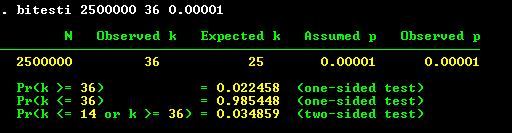
33 X ,500, X 0.05 Pr(k >= 36)

34 16

37 8 4 active, 5 inactive 0.2 active 0.0, 0.1, 0.2, , 1.0 accept P 0.2 active (0.99)

38 Operating Characteristic Curve (OC) N=8, p = 0.2 Pregnant probability of accept cumulative

39 18 19

40 Operating Characteristic Curve (OC) 0.0, 0.1, 0.2, , 1.0 accept P=0 P=0.1 P=0.2 P=0.3 P=0.4 P=0. 5 P=0. 6 P=0. 7 P=0. 8 P=0. 9 P=

41 8 4 accept accept OK accept accept accept accept 19 Operating Characteristic Curve (OC) OC (two stage screening)

42 Operating Characteristic Curve (OC) 1 accept 0 0 true 1 Cf. two stage screening 19

43 Poisson distribution binomial situation binomial distribution Poisson person-time Poisson distribution variance = np(1-p) Poisson p 0 1-p variance = np = mean 21

44 p 0, 1 p = 1, mean = variance = np Poisson Binomial 20

45 Poisson distribution 2 independence assumption B A Poisson Stationary assumption Poisson 1 1 Poisson Hazard model Poisson

46 Poisson Distribution P X x e λ λ x /x! 0 < x < infinity e= p 0, 1 p 1 mean = variance = np 21

47 l = np = 10,000 x = 2.4 P(X=4) = e-2.4 (2.4)4 / 4! = l = np = 3 P(X=x) = (x 3) / 3 > (p=0.05) X = 6 6

こんにちは由美子です

こんにちは由美子です 1 2 . sum Variable Obs Mean Std. Dev. Min Max ---------+----------------------------------------------------- var1 13.4923077.3545926.05 1.1 3 3 3 0.71 3 x 3 C 3 = 0.3579 2 1 0.71 2 x 0.29 x 3 C 2 = 0.4386