表題.PDF
|
|
|
- しほこ しどり
- 5 years ago
- Views:
Transcription
1 1P 94P
2
3
4 Ra : : g : C : : Pr : : Nu : : h : B :
5
6
7 ( )
")
8 DC (Bau [1])
9 : u = u(t) (1) 1 : u& = Raρ T cos( θ) dθ Pu (2) π 2 T T : T & = u + β + [ T (, t) T ] 2 W θ θ θ (3) -
10 T W 0 ( t) + Wn ( t)sin( nθ) n= 1 ( θ, t) = W (4) T ( θ, t) = n= 1 S n ( t)sin( nθ) + Cn ( t) + C ( t) cos( nθ) n (5) (4),(5) (1),(3) u& = c u p (6) c& = us c (7) s& uc s Ra[ 1+ εf ( t)] (8) =0 (6) (8) (Lorenz [3]) (Lorenz [3])
11 (Lorenz [3]) ( ) Lorenz equations : x& =σ( y x) (9) y& = rx y xz (10) z & = bz + xy (11)
12
13


14
15
16


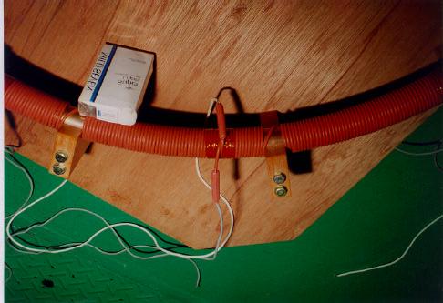
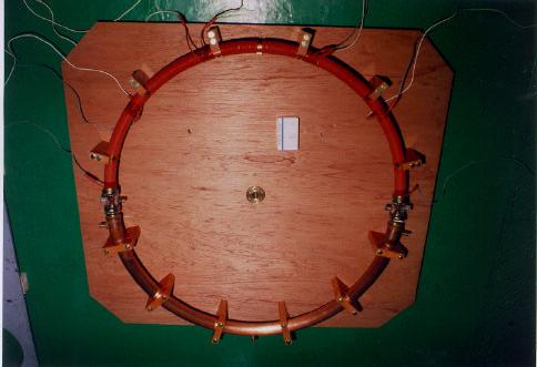
17 780mm

18

19 3 l/min 15 l/min

20 TakadaRiken TR DIGITAL MULUTIMETER ADVANTEST R6511 DIGITAL MULTIMETER TakadaRiken TR UNIVERSAL SCANNER

21 YEW TYPE3056 PEN RECORDER
22


23 RIKO SLIDE TRANS TYPE RSD-10A CAP 1KVA INPUT 100V
24
25
26
27 1. 25mm 20mm
28
29
30 760m 10mm 10mm left bottom right
31
32
33
34
35
36
37
38
39 5W 20 temperature( ) right bottom left time(sec) 4000 Fig4.2
40 20W 22 temperature( ) 20 left bottom right time(sec) Fig4.3
41 21 30W bottom temperature( ) left right time(sec) Fig4.4
42 30W 2 22 right temperature( ) bottom left time(sec) Fig4.5
43 40W 22 left temperature( ) bottom 19 right time(sec) 4000 Fig4.6
44 23 40W 22 left temperature( ) bottom 19 right time(sec) Fig4.7
45 50W 22 right temperature( ) 20 bottom left time(sec) 3000 Fig4.8
46 55W left 22 temperature( ) 20 bottom 18 right time(sec) Fig4.9
47 60W left 22 temperature( ) 20 bottom 18 right time(sec) Fig4.10
48 65W 24 right temperature( ) bottom left time(sec) 2000 Fig4.11
49 65W 24 right temperature( ) bottom left time(sec) 2000 Fig4.11
50 75W 24 temperature( ) right bottom left time(sec) 3000 Fig4.12
51 75W 24 temperature( ) right bottom left time(sec) Fig4.13
52 100W 26 right temperature( ) bottom left time(sec) Fig4.14
53 100W 26 right temperature( ) bottom left time(sec) Fig4.16
54 200W 30 right temperature( ) left bottom time(sec) Fig4.17
55 30 200W right temperature( ) 25 bottom left time(sec) Fig4.18
56 300W 35 right temperature( ) left bottom time(sec) Fig4.19
57 W right temperature( ) bottom left time(sec) Fig4.20
58 40 500W right temperature( ) 30 bottom left time(sec) Fig4.21
59 500W temperature( ) right bottom 26 left time(sec) Fig4.22
60 45 800W right 40 temperature( ) 35 bottom 30 left time(sec) Fig4.23
61 45 800W right 40 temperature( ) 35 bottom 30 left time(sec) Fig4.24
62 50 right 1000W 45 temperature( ) bottom 30 left time(sec) Fig4.25
63 W 45 right temperature( ) bottom left time(sec) Fig4.26
64 23 40W temperature( ) time(sec) Fig4.27
65 W temperature( ) time(sec) Fig4.28
66 24 60W 1 temperature( ) time(sec) Fig4.29
67 24 60W 1 temperature( ) time(sec) Fig4.30
68 70W temperature( ) time(sec) Fig4.31
69 100W temperature( ) time(sec) 680 Fig4.32
70 25 200W 3 temperature( ) time(sec) Fig4.33
71 400W temperature( ) time(sec) Fig4.34
72 50W frequency(hz) Fig4.35
73 50W 80 l 60 b r frequency(hz) Fig4.36
74 200 60W frequency(hz) Fig4.37
75 200 60W frequency(hz) Fig4.38
76 200 60W b 100 r l frequency(hz) Fig4.39
77 75W 60 r 40 b 20 l frequency(hz) Fig4.40
78
79
80 [1]Haim H.Bau and YuZou Wang, Chaos: A Heat Transfer Perspective, Annual Review of Heat Transfer [2]P.Wealander, On the Oscillatory Instability of Differentially Heated Fluid loops, J.Fluid Mech.,vol29,pp.17-30,1967. [3]Edward N Lorenz, Deterministic Nonperiodic Flow, J Atmospheric Sci.,vol.20,pp ,1963. [4],,
81 Eq: %0i*X^i (i=0-9) %00 = e+00 %01 = e+01 %02 = e+01 %03 = e+01 %04 = e+01 %05 = e+01 %06 = e+00 %07 = e+00 %08 = e-01 %09 = e-03 points = 16 <DY^2> = e-01 r or R = e-01
82 Eq: %0i*X^i (i=0-9) %00 = e+00 %01 = e+01 %02 = e+01 %03 = e+01 %04 = e+01 %05 = e+01 %06 = e+00 %07 = e+00 %08 = e-01 %09 = e-03 points = 16 <DY^2> = e-01 r or R = e-01
83 Eq: %0i*X^i (i=0-9) %00 = e+00 %01 = e+01 %02 = e+01 %03 = e+01 %04 = e+01 %05 = e+01 %06 = e+00 %07 = e+00 %08 = e-01 %09 = e-03 points = 16 <DY^2> = e-01 r or R = e-01
84 Eq: %0i*X^i (i=0-9) %00 = e+00 %01 = e+01 %02 = e+01 %03 = e+01 %04 = e+01 %05 = e+01 %06 = e+00 %07 = e+00 %08 = e-01 %09 = e-03 points = 16 <DY^2> = e-01 r or R = e-01
85 Eq: %0i*X^i (i=0-9) %00 = e+00 %01 = e+01 %02 = e+01 %03 = e+01 %04 = e+01 %05 = e+01 %06 = e+00 %07 = e+00 %08 = e-01 %09 = e-03 points = 16 <DY^2> = e-01 r or R = e-01
86 Eq: %0i*X^i (i=0-9) %00 = e+00 %01 = e+01 %02 = e+01 %03 = e+01 %04 = e+01 %05 = e+01 %06 = e+00 %07 = e+00 %08 = e-01 %09 = e-03 points = 16 <DY^2> = e-01 r or R = e-01
87
88 1 100 ( ) (mv)
89 2 100 ( ) (mv)
90 4 100 ( ) (mv)
91 4 100 ( ) (mv)
92 5 100 ( ) (mv)
93 6 100 ( ) (mv)
94 1P 94P
66 σ σ (8.1) σ = 0 0 σd = 0 (8.2) (8.2) (8.1) E ρ d = 0... d = 0 (8.3) d 1 NN K K 8.1 d σd σd M = σd = E 2 d (8.4) ρ 2 d = I M = EI ρ 1 ρ = M EI ρ EI
 σ = 0 0 σd = 0 (8.2) (8.2) (8.1) E ρ d = 0... d = 0 (8.3) d 1 NN K K 8.1 d σd σd M = σd = E 2 d (8.4) ρ 2 d = I M = EI ρ 1 ρ = M EI ρ EI") 65 8. K 8 8 7 8 K 6 7 8 K 6 M Q σ (6.4) M O ρ dθ D N d N 1 P Q B C (1 + ε)d M N N h 2 h 1 ( ) B (+) M 8.1: σ = E ρ (E, 1/ρ ) (8.1) 66 σ σ (8.1) σ = 0 0 σd = 0 (8.2) (8.2) (8.1) E ρ d = 0... d = 0 (8.3)
65 8. K 8 8 7 8 K 6 7 8 K 6 M Q σ (6.4) M O ρ dθ D N d N 1 P Q B C (1 + ε)d M N N h 2 h 1 ( ) B (+) M 8.1: σ = E ρ (E, 1/ρ ) (8.1) 66 σ σ (8.1) σ = 0 0 σd = 0 (8.2) (8.2) (8.1) E ρ d = 0... d = 0 (8.3)
charpter0.PDF
 Kutateladze Zuber C 0 C 1 r eq q CHF A v /A w A v /A w q CHF [1] [2] q CHF A v /A w [3] [4] A v : A w : A : g : H fg : Q : q : q CHF : T : T 1 : T 2 : T 3 : c 100 T 4 : c 100 T b : T sat : T w : t : V

JKR Point loading of an elastic half-space 2 3 Pressure applied to a circular region Boussinesq, n =
 JKR 17 9 15 1 Point loading of an elastic half-space Pressure applied to a circular region 4.1 Boussinesq, n = 1.............................. 4. Hertz, n = 1.................................. 6 4 Hertz
1 I 1.1 ± e = = - = C C MKSA [m], [Kg] [s] [A] 1C 1A 1 MKSA 1C 1C +q q +q q 1
![1 I 1.1 ± e = = - = C C MKSA [m], [Kg] [s] [A] 1C 1A 1 MKSA 1C 1C +q q +q q 1](/thumbs/94/121802164.jpg "1 I 1.1 ± e = = - = C C MKSA [m], [Kg] [s] [A] 1C 1A 1 MKSA 1C 1C +q q +q q 1") 1 I 1.1 ± e = = - =1.602 10 19 C C MKA [m], [Kg] [s] [A] 1C 1A 1 MKA 1C 1C +q q +q q 1 1.1 r 1,2 q 1, q 2 r 12 2 q 1, q 2 2 F 12 = k q 1q 2 r 12 2 (1.1) k 2 k 2 ( r 1 r 2 ) ( r 2 r 1 ) q 1 q 2 (q 1 q 2
1 I 1.1 ± e = = - =1.602 10 19 C C MKA [m], [Kg] [s] [A] 1C 1A 1 MKA 1C 1C +q q +q q 1 1.1 r 1,2 q 1, q 2 r 12 2 q 1, q 2 2 F 12 = k q 1q 2 r 12 2 (1.1) k 2 k 2 ( r 1 r 2 ) ( r 2 r 1 ) q 1 q 2 (q 1 q 2
報告書
 1 2 3 4 5 6 7 or 8 9 10 11 12 13 14 15 16 17 18 19 20 21 22 2.65 2.45 2.31 2.30 2.29 1.95 1.79 23 24 25 26 27 28 29 30 31 32 33 34 35 36 37 38 39 40 41 42 43 44 45 46 47 60 55 60 75 25 23 6064 65 60 1015
Shunsuke Kobayashi 1 [6] [11] [7] u t = D 2 u 1 x 2 + f(u, v) + s L u(t, x)dx, L x (0.L), t > 0, Neumann 0 v t = D 2 v 2 + g(u, v), x (0, L), t > 0. x
![Shunsuke Kobayashi 1 [6] [11] [7] u t = D 2 u 1 x 2 + f(u, v) + s L u(t, x)dx, L x (0.L), t > 0, Neumann 0 v t = D 2 v 2 + g(u, v), x (0, L), t > 0. x](/thumbs/97/133795870.jpg "Shunsuke Kobayashi 1 [6] [11] [7] u t = D 2 u 1 x 2 + f(u, v) + s L u(t, x)dx, L x (0.L), t > 0, Neumann 0 v t = D 2 v 2 + g(u, v), x (0, L), t > 0. x") Shunsuke Kobayashi [6] [] [7] u t = D 2 u x 2 + fu, v + s L ut, xdx, L x 0.L, t > 0, Neumann 0 v t = D 2 v 2 + gu, v, x 0, L, t > 0. x2 u u v t, 0 = t, L = 0, x x. v t, 0 = t, L = 0.2 x x ut, x R vt, x
Shunsuke Kobayashi [6] [] [7] u t = D 2 u x 2 + fu, v + s L ut, xdx, L x 0.L, t > 0, Neumann 0 v t = D 2 v 2 + gu, v, x 0, L, t > 0. x2 u u v t, 0 = t, L = 0, x x. v t, 0 = t, L = 0.2 x x ut, x R vt, x

A
 A05-132 2010 2 11 1 1 3 1.1.......................................... 3 1.2..................................... 3 1.3..................................... 3 2 4 2.1............................... 4 2.2
120 9 I I 1 I 2 I 1 I 2 ( a) ( b) ( c ) I I 2 I 1 I ( d) ( e) ( f ) 9.1: Ampère (c) (d) (e) S I 1 I 2 B ds = µ 0 ( I 1 I 2 ) I 1 I 2 B ds =0. I 1 I 2
 ( b) ( c ) I I 2 I 1 I ( d) ( e) ( f ) 9.1: Ampère (c) (d) (e) S I 1 I 2 B ds = µ 0 ( I 1 I 2 ) I 1 I 2 B ds =0. I 1 I 2") 9 E B 9.1 9.1.1 Ampère Ampère Ampère s law B S µ 0 B ds = µ 0 j ds (9.1) S rot B = µ 0 j (9.2) S Ampère Biot-Savart oulomb Gauss Ampère rot B 0 Ampère µ 0 9.1 (a) (b) I B ds = µ 0 I. I 1 I 2 B ds = µ 0
9 E B 9.1 9.1.1 Ampère Ampère Ampère s law B S µ 0 B ds = µ 0 j ds (9.1) S rot B = µ 0 j (9.2) S Ampère Biot-Savart oulomb Gauss Ampère rot B 0 Ampère µ 0 9.1 (a) (b) I B ds = µ 0 I. I 1 I 2 B ds = µ 0
Microsoft Word - ‚²‰ÆŸ_Ł¶−®’¬.doc
 1 1 75 1 4 81 1 3 4 5..5 6 3 1 4 5 1 6 7..5mm 8.1. C.1 ( ).5 ( ) ( ) 3. ( ).5. 1..5 1-131 TEACDR-F1 khz 648frame/sec 9 Hot Film Probe Anemometer Stabilizer Digital Recorder Video Compressor Camera Flow
q π =0 Ez,t =ε σ {e ikz ωt e ikz ωt } i/ = ε σ sinkz ωt 5.6 x σ σ *105 q π =1 Ez,t = 1 ε σ + ε π {e ikz ωt e ikz ωt } i/ = 1 ε σ + ε π sinkz ωt 5.7 σ
 H k r,t= η 5 Stokes X k, k, ε, ε σ π X Stokes 5.1 5.1.1 Maxwell H = A A *10 A = 1 c A t 5.1 A kη r,t=ε η e ik r ωt 5. k ω ε η k η = σ, π ε σ, ε π σ π A k r,t= q η A kη r,t+qηa kηr,t 5.3 η q η E = 1 c A
Gmech08.dvi
 63 6 6.1 6.1.1 v = v 0 =v 0x,v 0y, 0) t =0 x 0,y 0, 0) t x x 0 + v 0x t v x v 0x = y = y 0 + v 0y t, v = v y = v 0y 6.1) z 0 0 v z yv z zv y zv x xv z xv y yv x = 0 0 x 0 v 0y y 0 v 0x 6.) 6.) 6.1) 6.)
(1) 3 A B E e AE = e AB OE = OA + e AB = (1 35 e ) e OE z 1 1 e E xy e = 0 e = 5 OE = ( 2 0 0) E ( 2 0 0) (2) 3 E P Q k EQ = k EP E y 0
 3 A B E e AE = e AB OE = OA + e AB = (1 35 e ) e OE z 1 1 e E xy e = 0 e = 5 OE = ( 2 0 0) E ( 2 0 0) (2) 3 E P Q k EQ = k EP E y 0") (1) 3 A B E e AE = e AB OE = OA + e AB = (1 35 e 0 1 15 ) e OE z 1 1 e E xy 5 1 1 5 e = 0 e = 5 OE = ( 2 0 0) E ( 2 0 0) (2) 3 E P Q k EQ = k EP E y 0 Q y P y k 2 M N M( 1 0 0) N(1 0 0) 4 P Q M N C EP
(1) 3 A B E e AE = e AB OE = OA + e AB = (1 35 e 0 1 15 ) e OE z 1 1 e E xy 5 1 1 5 e = 0 e = 5 OE = ( 2 0 0) E ( 2 0 0) (2) 3 E P Q k EQ = k EP E y 0 Q y P y k 2 M N M( 1 0 0) N(1 0 0) 4 P Q M N C EP
(Compton Scattering) Beaming 1 exp [i (k x ωt)] k λ k = 2π/λ ω = 2πν k = ω/c k x ωt ( ω ) k α c, k k x ωt η αβ k α x β diag( + ++) x β = (ct, x) O O x
![(Compton Scattering) Beaming 1 exp [i (k x ωt)] k λ k = 2π/λ ω = 2πν k = ω/c k x ωt ( ω ) k α c, k k x ωt η αβ k α x β diag( + ++) x β = (ct, x) O O x](/thumbs/104/162595168.jpg "(Compton Scattering) Beaming 1 exp [i (k x ωt)] k λ k = 2π/λ ω = 2πν k = ω/c k x ωt ( ω ) k α c, k k x ωt η αβ k α x β diag( + ++) x β = (ct, x) O O x") Compton Scattering Beaming exp [i k x ωt] k λ k π/λ ω πν k ω/c k x ωt ω k α c, k k x ωt η αβ k α x β diag + ++ x β ct, x O O x O O v k α k α β, γ k γ k βk, k γ k + βk k γ k k, k γ k + βk 3 k k 4 k 3 k
Compton Scattering Beaming exp [i k x ωt] k λ k π/λ ω πν k ω/c k x ωt ω k α c, k k x ωt η αβ k α x β diag + ++ x β ct, x O O x O O v k α k α β, γ k γ k βk, k γ k + βk k γ k k, k γ k + βk 3 k k 4 k 3 k
all.dvi
 38 5 Cauchy.,,,,., σ.,, 3,,. 5.1 Cauchy (a) (b) (a) (b) 5.1: 5.1. Cauchy 39 F Q Newton F F F Q F Q 5.2: n n ds df n ( 5.1). df n n df(n) df n, t n. t n = df n (5.1) ds 40 5 Cauchy t l n mds df n 5.3: t
18 2 F 12 r 2 r 1 (3) Coulomb km Coulomb M = kg F G = ( ) ( ) ( ) 2 = [N]. Coulomb
![18 2 F 12 r 2 r 1 (3) Coulomb km Coulomb M = kg F G = ( ) ( ) ( ) 2 = [N]. Coulomb](/thumbs/93/114079295.jpg "18 2 F 12 r 2 r 1 (3) Coulomb km Coulomb M = kg F G = ( ) ( ) ( ) 2 = [N]. Coulomb") r 1 r 2 r 1 r 2 2 Coulomb Gauss Coulomb 2.1 Coulomb 1 2 r 1 r 2 1 2 F 12 2 1 F 21 F 12 = F 21 = 1 4πε 0 1 2 r 1 r 2 2 r 1 r 2 r 1 r 2 (2.1) Coulomb ε 0 = 107 4πc 2 =8.854 187 817 10 12 C 2 N 1 m 2 (2.2)
r 1 r 2 r 1 r 2 2 Coulomb Gauss Coulomb 2.1 Coulomb 1 2 r 1 r 2 1 2 F 12 2 1 F 21 F 12 = F 21 = 1 4πε 0 1 2 r 1 r 2 2 r 1 r 2 r 1 r 2 (2.1) Coulomb ε 0 = 107 4πc 2 =8.854 187 817 10 12 C 2 N 1 m 2 (2.2)

9 2 1 f(x, y) = xy sin x cos y x y cos y y x sin x d (x, y) = y cos y (x sin x) = y cos y(sin x + x cos x) x dx d (x, y) = x sin x (y cos y) = x sin x
 = xy sin x cos y x y cos y y x sin x d (x, y) = y cos y (x sin x) = y cos y(sin x + x cos x) x dx d (x, y) = x sin x (y cos y) = x sin x") 2009 9 6 16 7 1 7.1 1 1 1 9 2 1 f(x, y) = xy sin x cos y x y cos y y x sin x d (x, y) = y cos y (x sin x) = y cos y(sin x + x cos x) x dx d (x, y) = x sin x (y cos y) = x sin x(cos y y sin y) y dy 1 sin
2009 9 6 16 7 1 7.1 1 1 1 9 2 1 f(x, y) = xy sin x cos y x y cos y y x sin x d (x, y) = y cos y (x sin x) = y cos y(sin x + x cos x) x dx d (x, y) = x sin x (y cos y) = x sin x(cos y y sin y) y dy 1 sin
e a b a b b a a a 1 a a 1 = a 1 a = e G G G : x ( x =, 8, 1 ) x 1,, 60 θ, ϕ ψ θ G G H H G x. n n 1 n 1 n σ = (σ 1, σ,..., σ N ) i σ i i n S n n = 1,,
 x 1,, 60 θ, ϕ ψ θ G G H H G x. n n 1 n 1 n σ = (σ 1, σ,..., σ N ) i σ i i n S n n = 1,,") 01 10 18 ( ) 1 6 6 1 8 8 1 6 1 0 0 0 0 1 Table 1: 10 0 8 180 1 1 1. ( : 60 60 ) : 1. 1 e a b a b b a a a 1 a a 1 = a 1 a = e G G G : x ( x =, 8, 1 ) x 1,, 60 θ, ϕ ψ θ G G H H G x. n n 1 n 1 n σ = (σ 1,
01 10 18 ( ) 1 6 6 1 8 8 1 6 1 0 0 0 0 1 Table 1: 10 0 8 180 1 1 1. ( : 60 60 ) : 1. 1 e a b a b b a a a 1 a a 1 = a 1 a = e G G G : x ( x =, 8, 1 ) x 1,, 60 θ, ϕ ψ θ G G H H G x. n n 1 n 1 n σ = (σ 1,
untitled
 1 ( 12 11 44 7 20 10 10 1 1 ( ( 2 10 46 11 10 10 5 8 3 2 6 9 47 2 3 48 4 2 2 ( 97 12 ) 97 12 -Spencer modulus moduli (modulus of elasticity) modulus (le) module modulus module 4 b θ a q φ p 1: 3 (le) module
meiji_resume_1.PDF
 β β β (q 1,q,..., q n ; p 1, p,..., p n ) H(q 1,q,..., q n ; p 1, p,..., p n ) Hψ = εψ ε k = k +1/ ε k = k(k 1) (x, y, z; p x, p y, p z ) (r; p r ), (θ; p θ ), (ϕ; p ϕ ) ε k = 1/ k p i dq i E total = E
c y /2 ddy = = 2π sin θ /2 dθd /2 [ ] 2π cos θ d = log 2 + a 2 d = log 2 + a 2 = log 2 + a a 2 d d + 2 = l
![c y /2 ddy = = 2π sin θ /2 dθd /2 [ ] 2π cos θ d = log 2 + a 2 d = log 2 + a 2 = log 2 + a a 2 d d + 2 = l](/thumbs/85/91372642.jpg "c y /2 ddy = = 2π sin θ /2 dθd /2 [ ] 2π cos θ d = log 2 + a 2 d = log 2 + a 2 = log 2 + a a 2 d d + 2 = l") c 28. 2, y 2, θ = cos θ y = sin θ 2 3, y, 3, θ, ϕ = sin θ cos ϕ 3 y = sin θ sin ϕ 4 = cos θ 5.2 2 e, e y 2 e, e θ e = cos θ e sin θ e θ 6 e y = sin θ e + cos θ e θ 7.3 sgn sgn = = { = + > 2 < 8.4 a b 2
c 28. 2, y 2, θ = cos θ y = sin θ 2 3, y, 3, θ, ϕ = sin θ cos ϕ 3 y = sin θ sin ϕ 4 = cos θ 5.2 2 e, e y 2 e, e θ e = cos θ e sin θ e θ 6 e y = sin θ e + cos θ e θ 7.3 sgn sgn = = { = + > 2 < 8.4 a b 2
2.5 (Gauss) (flux) v(r)( ) S n S v n v n (1) v n S = v n S = v S, n S S. n n S v S v Minoru TANAKA (Osaka Univ.) I(2012), Sec p. 1/30
 (flux) v(r)( ) S n S v n v n (1) v n S = v n S = v S, n S S. n n S v S v Minoru TANAKA (Osaka Univ.) I(2012), Sec p. 1/30") 2.5 (Gauss) 2.5.1 (flux) v(r)( ) n v n v n (1) v n = v n = v, n. n n v v I(2012), ec. 2. 5 p. 1/30 i (2) lim v(r i ) i = v(r) d. i 0 i (flux) I(2012), ec. 2. 5 p. 2/30 2.5.2 ( ) ( ) q 1 r 2 E 2 q r 1 E
2.5 (Gauss) 2.5.1 (flux) v(r)( ) n v n v n (1) v n = v n = v, n. n n v v I(2012), ec. 2. 5 p. 1/30 i (2) lim v(r i ) i = v(r) d. i 0 i (flux) I(2012), ec. 2. 5 p. 2/30 2.5.2 ( ) ( ) q 1 r 2 E 2 q r 1 E

R¤Çʬ¤«¤ëÎÏ³Ø·Ï - ¡Áʬ´ô¤ÎÍͻҤò²Ä»ë²½¤·¤Æ¤ß¤ë¡Á
 .... R 2009 3 1 ( ) R 2009 3 1 1 / 23 : ( )!, @tkf, id:tkf41, (id:artk ) : 4 1 : http://arataka.wordpress.com : Python, C/C++, PHP, Javascript R : / ( ) R 2009 3 1 2 / 23 R? R! ( ) R 2009 3 1 3 / 23 =

Gmech08.dvi
 145 13 13.1 13.1.1 0 m mg S 13.1 F 13.1 F /m S F F 13.1 F mg S F F mg 13.1: m d2 r 2 = F + F = 0 (13.1) 146 13 F = F (13.2) S S S S S P r S P r r = r 0 + r (13.3) r 0 S S m d2 r 2 = F (13.4) (13.3) d 2
TOP URL 1
 TOP URL http://amonphys.web.fc.com/ 1 19 3 19.1................... 3 19.............................. 4 19.3............................... 6 19.4.............................. 8 19.5.............................
II (10 4 ) 1. p (x, y) (a, b) ε(x, y; a, b) 0 f (x, y) f (a, b) A, B (6.5) y = b f (x, b) f (a, b) x a = A + ε(x, b; a, b) x a 2 x a 0 A = f x (
 1. p (x, y) (a, b) ε(x, y; a, b) 0 f (x, y) f (a, b) A, B (6.5) y = b f (x, b) f (a, b) x a = A + ε(x, b; a, b) x a 2 x a 0 A = f x (") II (1 4 ) 1. p.13 1 (x, y) (a, b) ε(x, y; a, b) f (x, y) f (a, b) A, B (6.5) y = b f (x, b) f (a, b) x a = A + ε(x, b; a, b) x a x a A = f x (a, b) y x 3 3y 3 (x, y) (, ) f (x, y) = x + y (x, y) = (, )
II (1 4 ) 1. p.13 1 (x, y) (a, b) ε(x, y; a, b) f (x, y) f (a, b) A, B (6.5) y = b f (x, b) f (a, b) x a = A + ε(x, b; a, b) x a x a A = f x (a, b) y x 3 3y 3 (x, y) (, ) f (x, y) = x + y (x, y) = (, )
#A A A F, F d F P + F P = d P F, F y P F F x A.1 ( α, 0), (α, 0) α > 0) (x, y) (x + α) 2 + y 2, (x α) 2 + y 2 d (x + α)2 + y 2 + (x α) 2 + y 2 =
, (α, 0) α > 0) (x, y) (x + α) 2 + y 2, (x α) 2 + y 2 d (x + α)2 + y 2 + (x α) 2 + y 2 =") #A A A. F, F d F P + F P = d P F, F P F F A. α, 0, α, 0 α > 0, + α +, α + d + α + + α + = d d F, F 0 < α < d + α + = d α + + α + = d d α + + α + d α + = d 4 4d α + = d 4 8d + 6 http://mth.cs.kitmi-it.c.jp/
#A A A. F, F d F P + F P = d P F, F P F F A. α, 0, α, 0 α > 0, + α +, α + d + α + + α + = d d F, F 0 < α < d + α + = d α + + α + = d d α + + α + d α + = d 4 4d α + = d 4 8d + 6 http://mth.cs.kitmi-it.c.jp/
知能科学:ニューラルネットワーク
 2 3 4 (Neural Network) (Deep Learning) (Deep Learning) ( x x = ax + b x x x ? x x x w σ b = σ(wx + b) x w b w b .2.8.6 σ(x) = + e x.4.2 -.2 - -5 5 x w x2 w2 σ x3 w3 b = σ(w x + w 2 x 2 + w 3 x 3 + b) x,
知能科学:ニューラルネットワーク
 2 3 4 (Neural Network) (Deep Learning) (Deep Learning) ( x x = ax + b x x x ? x x x w σ b = σ(wx + b) x w b w b .2.8.6 σ(x) = + e x.4.2 -.2 - -5 5 x w x2 w2 σ x3 w3 b = σ(w x + w 2 x 2 + w 3 x 3 + b) x,

29
 9 .,,, 3 () C k k C k C + C + C + + C 8 + C 9 + C k C + C + C + C 3 + C 4 + C 5 + + 45 + + + 5 + + 9 + 4 + 4 + 5 4 C k k k ( + ) 4 C k k ( k) 3 n( ) n n n ( ) n ( ) n 3 ( ) 3 3 3 n 4 ( ) 4 4 4 ( ) n n

 http://www.ns.kogakuin.ac.jp/~ft13389/lecture/physics1a2b/ pdf I 1 1 1.1 ( ) 1. 30 m µm 2. 20 cm km 3. 10 m 2 cm 2 4. 5 cm 3 km 3 5. 1 6. 1 7. 1 1.2 ( ) 1. 1 m + 10 cm 2. 1 hr + 6400 sec 3. 3.0 10 5 kg
12
 12 1 2 3 4 5 6 1.2 AFRP (3.4.1)(3.4.3) ht M = 1.2M By0 M Ty0 h A n MBy0 h B AF p = 1000 = t AF AAF b 7 / 8 AF B M σ AFb h (tf m) (m) M T y0 (tf m) h T (m) M (tf m) AAF AFRPcm 2 σafb AFRPkgf/cm 2 σ AFb


 K E N Z U 2012 7 16 HP M. 1 1 4 1.1 3.......................... 4 1.2................................... 4 1.2.1..................................... 4 1.2.2.................................... 5................................


微分積分 サンプルページ この本の定価 判型などは, 以下の URL からご覧いただけます. このサンプルページの内容は, 初版 1 刷発行時のものです.
 微分積分 サンプルページ この本の定価 判型などは, 以下の URL からご覧いただけます. ttp://www.morikita.co.jp/books/mid/00571 このサンプルページの内容は, 初版 1 刷発行時のものです. i ii 014 10 iii [note] 1 3 iv 4 5 3 6 4 x 0 sin x x 1 5 6 z = f(x, y) 1 y = f(x)
 1 3 1.1.......................... 3 1............................... 3 1.3....................... 5 1.4.......................... 6 1.5........................ 7 8.1......................... 8..............................
untitled
 20 7 1 22 7 1 1 2 3 7 8 9 10 11 13 14 15 17 18 19 21 22 - 1 - - 2 - - 3 - - 4 - 50 200 50 200-5 - 50 200 50 200 50 200 - 6 - - 7 - () - 8 - (XY) - 9 - 112-10 - - 11 - - 12 - - 13 - - 14 - - 15 - - 16 -
untitled
 19 1 19 19 3 8 1 19 1 61 2 479 1965 64 1237 148 1272 58 183 X 1 X 2 12 2 15 A B 5 18 B 29 X 1 12 10 31 A 1 58 Y B 14 1 25 3 31 1 5 5 15 Y B 1 232 Y B 1 4235 14 11 8 5350 2409 X 1 15 10 10 B Y Y 2 X 1 X

 1 2 3 4 5 1 1 136 2 137 2 1 1 138 2 1 2 139 140 141 142 3 143 3 144 145 4 1 2 146 3 4 147 5 1 2 3 148 1 2 149 3 5 1 2 150 3 151 1 152 2 153 6 1 2 154 3 155 4 1 156 2 3 4 5 157 7 1 2 3 4 158 5 159 6 8 1
,.,. 2, R 2, ( )., I R. c : I R 2, : (1) c C -, (2) t I, c (t) (0, 0). c(i). c (t)., c(t) = (x(t), y(t)) c (t) = (x (t), y (t)) : (1)
., I R. c : I R 2, : (1) c C -, (2) t I, c (t) (0, 0). c(i). c (t)., c(t) = (x(t), y(t)) c (t) = (x (t), y (t)) : (1)") ( ) 1., : ;, ;, ; =. ( ).,.,,,., 2.,.,,.,.,,., y = f(x), f ( ).,,.,.,., U R m, F : U R n, M, f : M R p M, p,, R m,,, R m. 2009 A tamaru math.sci.hiroshima-u.ac.jp 1 ,.,. 2, R 2, ( ).,. 2.1 2.1. I R. c
( ) 1., : ;, ;, ; =. ( ).,.,,,., 2.,.,,.,.,,., y = f(x), f ( ).,,.,.,., U R m, F : U R n, M, f : M R p M, p,, R m,,, R m. 2009 A tamaru math.sci.hiroshima-u.ac.jp 1 ,.,. 2, R 2, ( ).,. 2.1 2.1. I R. c
06佐々木雅哉_4C.indd
 3 2 3 2 4 5 56 57 3 2013 9 2012 16 19 62.2 17 2013 7 170 77 170 131 58 9 10 59 3 2 10 15 F 12 12 48 60 1 3 1 4 7 61 3 7 1 62 T C C T C C1 2 3 T C 1 C 1 T C C C T T C T C C 63 3 T 4 T C C T C C CN T C C
 21 2 26 i 1 1 1.1............................ 1 1.2............................ 3 2 9 2.1................... 9 2.2.......... 9 2.3................... 11 2.4....................... 12 3 15 3.1..........
Title 混合体モデルに基づく圧縮性流体と移動する固体の熱連成計算手法 Author(s) 鳥生, 大祐 ; 牛島, 省 Citation 土木学会論文集 A2( 応用力学 ) = Journal of Japan Civil Engineers, Ser. A2 (2017), 73 Issue
 鳥生, 大祐 ; 牛島, 省 Citation 土木学会論文集 A2( 応用力学 ) = Journal of Japan Civil Engineers, Ser. A2 (2017), 73 Issue") Title 混合体モデルに基づく圧縮性流体と移動する固体の熱連成計算手法 Author(s) 鳥生, 大祐 ; 牛島, 省 Citation 土木学会論文集 A2( 応用力学 ) = Journal of Japan Civil Engineers, Ser. A2 (2017), 73 Issue Date 2017 URL http://hdl.handle.net/2433/229150 Right
Title 混合体モデルに基づく圧縮性流体と移動する固体の熱連成計算手法 Author(s) 鳥生, 大祐 ; 牛島, 省 Citation 土木学会論文集 A2( 応用力学 ) = Journal of Japan Civil Engineers, Ser. A2 (2017), 73 Issue Date 2017 URL http://hdl.handle.net/2433/229150 Right
, 3, 6 = 3, 3,,,, 3,, 9, 3, 9, 3, 3, 4, 43, 4, 3, 9, 6, 6,, 0 p, p, p 3,..., p n N = p p p 3 p n + N p n N p p p, p 3,..., p n p, p,..., p n N, 3,,,,
 6,,3,4,, 3 4 8 6 6................................. 6.................................. , 3, 6 = 3, 3,,,, 3,, 9, 3, 9, 3, 3, 4, 43, 4, 3, 9, 6, 6,, 0 p, p, p 3,..., p n N = p p p 3 p n + N p n N p p p,
x = a 1 f (a r, a + r) f(a) r a f f(a) 2 2. (a, b) 2 f (a, b) r f(a, b) r (a, b) f f(a, b)
 f(a) r a f f(a) 2 2. (a, b) 2 f (a, b) r f(a, b) r (a, b) f f(a, b)") 2011 I 2 II III 17, 18, 19 7 7 1 2 2 2 1 2 1 1 1.1.............................. 2 1.2 : 1.................... 4 1.2.1 2............................... 5 1.3 : 2.................... 5 1.3.1 2.....................................
2011 I 2 II III 17, 18, 19 7 7 1 2 2 2 1 2 1 1 1.1.............................. 2 1.2 : 1.................... 4 1.2.1 2............................... 5 1.3 : 2.................... 5 1.3.1 2.....................................
85 4
 85 4 86 Copright c 005 Kumanekosha 4.1 ( ) ( t ) t, t 4.1.1 t Step! (Step 1) (, 0) (Step ) ±V t (, t) I Check! P P V t π 54 t = 0 + V (, t) π θ : = θ : π ) θ = π ± sin ± cos t = 0 (, 0) = sin π V + t +V
ma22-9 u ( v w) = u v w sin θê = v w sin θ u cos φ = = 2.3 ( a b) ( c d) = ( a c)( b d) ( a d)( b c) ( a b) ( c d) = (a 2 b 3 a 3 b 2 )(c 2 d 3 c 3 d
 = u v w sin θê = v w sin θ u cos φ = = 2.3 ( a b) ( c d) = ( a c)( b d) ( a d)( b c) ( a b) ( c d) = (a 2 b 3 a 3 b 2 )(c 2 d 3 c 3 d") A 2. x F (t) =f sin ωt x(0) = ẋ(0) = 0 ω θ sin θ θ 3! θ3 v = f mω cos ωt x = f mω (t sin ωt) ω t 0 = f ( cos ωt) mω x ma2-2 t ω x f (t mω ω (ωt ) 6 (ωt)3 = f 6m ωt3 2.2 u ( v w) = v ( w u) = w ( u v) ma22-9
A 2. x F (t) =f sin ωt x(0) = ẋ(0) = 0 ω θ sin θ θ 3! θ3 v = f mω cos ωt x = f mω (t sin ωt) ω t 0 = f ( cos ωt) mω x ma2-2 t ω x f (t mω ω (ωt ) 6 (ωt)3 = f 6m ωt3 2.2 u ( v w) = v ( w u) = w ( u v) ma22-9
( ) ( )
 ( )") 20 21 2 8 1 2 2 3 21 3 22 3 23 4 24 5 25 5 26 6 27 8 28 ( ) 9 3 10 31 10 32 ( ) 12 4 13 41 0 13 42 14 43 0 15 44 17 5 18 6 18 1 1 2 2 1 2 1 0 2 0 3 0 4 0 2 2 21 t (x(t) y(t)) 2 x(t) y(t) γ(t) (x(t) y(t))
20 21 2 8 1 2 2 3 21 3 22 3 23 4 24 5 25 5 26 6 27 8 28 ( ) 9 3 10 31 10 32 ( ) 12 4 13 41 0 13 42 14 43 0 15 44 17 5 18 6 18 1 1 2 2 1 2 1 0 2 0 3 0 4 0 2 2 21 t (x(t) y(t)) 2 x(t) y(t) γ(t) (x(t) y(t))
(1.2) T D = 0 T = D = 30 kn 1.2 (1.4) 2F W = 0 F = W/2 = 300 kn/2 = 150 kn 1.3 (1.9) R = W 1 + W 2 = = 1100 N. (1.9) W 2 b W 1 a = 0
 T D = 0 T = D = 30 kn 1.2 (1.4) 2F W = 0 F = W/2 = 300 kn/2 = 150 kn 1.3 (1.9) R = W 1 + W 2 = = 1100 N. (1.9) W 2 b W 1 a = 0") 1 1 1.1 1.) T D = T = D = kn 1. 1.4) F W = F = W/ = kn/ = 15 kn 1. 1.9) R = W 1 + W = 6 + 5 = 11 N. 1.9) W b W 1 a = a = W /W 1 )b = 5/6) = 5 cm 1.4 AB AC P 1, P x, y x, y y x 1.4.) P sin 6 + P 1 sin 45
1 1 1.1 1.) T D = T = D = kn 1. 1.4) F W = F = W/ = kn/ = 15 kn 1. 1.9) R = W 1 + W = 6 + 5 = 11 N. 1.9) W b W 1 a = a = W /W 1 )b = 5/6) = 5 cm 1.4 AB AC P 1, P x, y x, y y x 1.4.) P sin 6 + P 1 sin 45
05Mar2001_tune.dvi
 2001 3 5 COD 1 1.1 u d2 u + ku =0 (1) dt2 u = a exp(pt) (2) p = ± k (3) k>0k = ω 2 exp(±iωt) (4) k
2 1 x 1.1: v mg x (t) = v(t) mv (t) = mg 0 x(0) = x 0 v(0) = v 0 x(t) = x 0 + v 0 t 1 2 gt2 v(t) = v 0 gt t x = x 0 + v2 0 2g v2 2g 1.1 (x, v) θ
 = v(t) mv (t) = mg 0 x(0) = x 0 v(0) = v 0 x(t) = x 0 + v 0 t 1 2 gt2 v(t) = v 0 gt t x = x 0 + v2 0 2g v2 2g 1.1 (x, v) θ") 1 1 1.1 (Isaac Newton, 1642 1727) 1. : 2. ( ) F = ma 3. ; F a 2 t x(t) v(t) = x (t) v (t) = x (t) F 3 3 3 3 3 3 6 1 2 6 12 1 3 1 2 m 2 1 x 1.1: v mg x (t) = v(t) mv (t) = mg 0 x(0) = x 0 v(0) = v 0 x(t)
1 1 1.1 (Isaac Newton, 1642 1727) 1. : 2. ( ) F = ma 3. ; F a 2 t x(t) v(t) = x (t) v (t) = x (t) F 3 3 3 3 3 3 6 1 2 6 12 1 3 1 2 m 2 1 x 1.1: v mg x (t) = v(t) mv (t) = mg 0 x(0) = x 0 v(0) = v 0 x(t)
総研大恒星進化概要.dvi
 The Structure and Evolution of Stars I. Basic Equations. M r r =4πr2 ρ () P r = GM rρ. r 2 (2) r: M r : P and ρ: G: M r Lagrange r = M r 4πr 2 rho ( ) P = GM r M r 4πr. 4 (2 ) s(ρ, P ) s(ρ, P ) r L r T
. ev=,604k m 3 Debye ɛ 0 kt e λ D = n e n e Ze 4 ln Λ ν ei = 5.6π / ɛ 0 m/ e kt e /3 ν ei v e H + +e H ev Saha x x = 3/ πme kt g i g e n
 003...............................3 Debye................. 3.4................ 3 3 3 3. Larmor Cyclotron... 3 3................ 4 3.3.......... 4 3.3............ 4 3.3...... 4 3.3.3............ 5 3.4.........
( ) e + e ( ) ( ) e + e () ( ) e e Τ ( ) e e ( ) ( ) () () ( ) ( ) ( ) ( )
 e + e ( ) ( ) e + e () ( ) e e Τ ( ) e e ( ) ( ) () () ( ) ( ) ( ) ( )") n n (n) (n) (n) (n) n n ( n) n n n n n en1, en ( n) nen1 + nen nen1, nen ( ) e + e ( ) ( ) e + e () ( ) e e Τ ( ) e e ( ) ( ) () () ( ) ( ) ( ) ( ) ( n) Τ n n n ( n) n + n ( n) (n) n + n n n n n n n n
n n (n) (n) (n) (n) n n ( n) n n n n n en1, en ( n) nen1 + nen nen1, nen ( ) e + e ( ) ( ) e + e () ( ) e e Τ ( ) e e ( ) ( ) () () ( ) ( ) ( ) ( ) ( n) Τ n n n ( n) n + n ( n) (n) n + n n n n n n n n
変 位 変位とは 物体中のある点が変形後に 別の点に異動したときの位置の変化で あり ベクトル量である 変位には 物体の変形の他に剛体運動 剛体変位 が含まれている 剛体変位 P(x, y, z) 平行移動と回転 P! (x + u, y + v, z + w) Q(x + d x, y + dy,
 平行移動と回転 P! (x + u, y + v, z + w) Q(x + d x, y + dy,") 変 位 変位とは 物体中のある点が変形後に 別の点に異動したときの位置の変化で あり ベクトル量である 変位には 物体の変形の他に剛体運動 剛体変位 が含まれている 剛体変位 P(x, y, z) 平行移動と回転 P! (x + u, y + v, z + w) Q(x + d x, y + dy, z + dz) Q! (x + d x + u + du, y + dy + v + dv, z +
変 位 変位とは 物体中のある点が変形後に 別の点に異動したときの位置の変化で あり ベクトル量である 変位には 物体の変形の他に剛体運動 剛体変位 が含まれている 剛体変位 P(x, y, z) 平行移動と回転 P! (x + u, y + v, z + w) Q(x + d x, y + dy, z + dz) Q! (x + d x + u + du, y + dy + v + dv, z +
TOP URL 1
 TOP URL http://amonphys.web.fc.com/ 3.............................. 3.............................. 4.3 4................... 5.4........................ 6.5........................ 8.6...........................7
Part () () Γ Part ,
 () Γ Part ,") Contents a 6 6 6 6 6 6 6 7 7. 8.. 8.. 8.3. 8 Part. 9. 9.. 9.. 3. 3.. 3.. 3 4. 5 4.. 5 4.. 9 4.3. 3 Part. 6 5. () 6 5.. () 7 5.. 9 5.3. Γ 3 6. 3 6.. 3 6.. 3 6.3. 33 Part 3. 34 7. 34 7.. 34 7.. 34 8. 35
Contents a 6 6 6 6 6 6 6 7 7. 8.. 8.. 8.3. 8 Part. 9. 9.. 9.. 3. 3.. 3.. 3 4. 5 4.. 5 4.. 9 4.3. 3 Part. 6 5. () 6 5.. () 7 5.. 9 5.3. Γ 3 6. 3 6.. 3 6.. 3 6.3. 33 Part 3. 34 7. 34 7.. 34 7.. 34 8. 35
2009 IA 5 I 22, 23, 24, 25, 26, (1) Arcsin 1 ( 2 (4) Arccos 1 ) 2 3 (2) Arcsin( 1) (3) Arccos 2 (5) Arctan 1 (6) Arctan ( 3 ) 3 2. n (1) ta
 Arcsin 1 ( 2 (4) Arccos 1 ) 2 3 (2) Arcsin( 1) (3) Arccos 2 (5) Arctan 1 (6) Arctan ( 3 ) 3 2. n (1) ta") 009 IA 5 I, 3, 4, 5, 6, 7 6 3. () Arcsin ( (4) Arccos ) 3 () Arcsin( ) (3) Arccos (5) Arctan (6) Arctan ( 3 ) 3. n () tan x (nπ π/, nπ + π/) f n (x) f n (x) fn (x) Arctan x () sin x [nπ π/, nπ +π/] g n
009 IA 5 I, 3, 4, 5, 6, 7 6 3. () Arcsin ( (4) Arccos ) 3 () Arcsin( ) (3) Arccos (5) Arctan (6) Arctan ( 3 ) 3. n () tan x (nπ π/, nπ + π/) f n (x) f n (x) fn (x) Arctan x () sin x [nπ π/, nπ +π/] g n
D v D F v/d F v D F η v D (3.2) (a) F=0 (b) v=const. D F v Newtonian fluid σ ė σ = ηė (2.2) ė kl σ ij = D ijkl ė kl D ijkl (2.14) ė ij (3.3) µ η visco
 (a) F=0 (b) v=const. D F v Newtonian fluid σ ė σ = ηė (2.2) ė kl σ ij = D ijkl ė kl D ijkl (2.14) ė ij (3.3) µ η visco") post glacial rebound 3.1 Viscosity and Newtonian fluid f i = kx i σ ij e kl ideal fluid (1.9) irreversible process e ij u k strain rate tensor (3.1) v i u i / t e ij v F 23 D v D F v/d F v D F η v D (3.2)
post glacial rebound 3.1 Viscosity and Newtonian fluid f i = kx i σ ij e kl ideal fluid (1.9) irreversible process e ij u k strain rate tensor (3.1) v i u i / t e ij v F 23 D v D F v/d F v D F η v D (3.2)
<967B92AC B82DC82BF82C382AD82E88C7689E68F912E706466>
 16m80m 16 4 1100 17 1 1 1 2 2 4 2 3 3 2 3 2 1 5 1 1 18 1/100 18 1 2 3 2~4 1 1 1 2 26 () 27 5 28 300 29 () 30 31 32 20229 5/30 - (83-2041) 68 2 2 1 7 1 1 4 7 7 2 1 1 2 4 1 2 181222 1 // 2 // 3 // 4 /
CG38.PDF
 ............3...3...6....6....8.....8.....4...9 3....9 3.... 3.3...4 3.4...36...39 4....39 4.....39 4.....4 4....49 4.....5 4.....57...64 5....64 5....66 5.3...68 5.4...7 5.5...77...8 6....8 6.....8 6.....83
 1 B64653 1 1 3.1....................................... 3.......................... 3..1.............................. 4................................ 4..3.............................. 5..4..............................
 155 13 2 15 B97176 1 1.1. 4 1.2. 5 1.2.1. 1.2.2. 1.3. 7 2. 2.1. 9 2.2. 1 2.3. 13 2.4. 16 3. 3.1. 3.1.1. 18 3.1.2. 26 3.1.3. 33 3.2. 3.2.1. 34 3.2.2. 5 4. 4.1. 52 4.2. 53 54 55 2 1 1.1 1.2 1.3 3 4 Fig.
2.4 ( ) ( B ) A B F (1) W = B A F dr. A F q dr f(x,y,z) A B Γ( ) Minoru TANAKA (Osaka Univ.) I(2011), Sec p. 1/30
 ( B ) A B F (1) W = B A F dr. A F q dr f(x,y,z) A B Γ( ) Minoru TANAKA (Osaka Univ.) I(2011), Sec p. 1/30") 2.4 ( ) 2.4.1 ( B ) A B F (1) W = B A F dr. A F q dr f(x,y,z) A B Γ( ) I(2011), Sec. 2. 4 p. 1/30 (2) Γ f dr lim f i r i. r i 0 i f i i f r i i i+1 (1) n i r i (3) F dr = lim F i n i r i. Γ r i 0 i n i
2.4 ( ) 2.4.1 ( B ) A B F (1) W = B A F dr. A F q dr f(x,y,z) A B Γ( ) I(2011), Sec. 2. 4 p. 1/30 (2) Γ f dr lim f i r i. r i 0 i f i i f r i i i+1 (1) n i r i (3) F dr = lim F i n i r i. Γ r i 0 i n i
2 1 κ c(t) = (x(t), y(t)) ( ) det(c (t), c x (t)) = det (t) x (t) y (t) y = x (t)y (t) x (t)y (t), (t) c (t) = (x (t)) 2 + (y (t)) 2. c (t) =
 = (x(t), y(t)) ( ) det(c (t), c x (t)) = det (t) x (t) y (t) y = x (t)y (t) x (t)y (t), (t) c (t) = (x (t)) 2 + (y (t)) 2. c (t) =") 1 1 1.1 I R 1.1.1 c : I R 2 (i) c C (ii) t I c (t) (0, 0) c (t) c(i) c c(t) 1.1.2 (1) (2) (3) (1) r > 0 c : R R 2 : t (r cos t, r sin t) (2) C f : I R c : I R 2 : t (t, f(t)) (3) y = x c : R R 2 : t (t,
1 1 1.1 I R 1.1.1 c : I R 2 (i) c C (ii) t I c (t) (0, 0) c (t) c(i) c c(t) 1.1.2 (1) (2) (3) (1) r > 0 c : R R 2 : t (r cos t, r sin t) (2) C f : I R c : I R 2 : t (t, f(t)) (3) y = x c : R R 2 : t (t,
main.dvi
 2 e jωt, 0 ωt < 2π 2.1 2.1.1 x(n) X(z) = x(n)z n (2.1) z z z = e σ+jωt = re jωt, r = e σ (2.2) ωt 0 2π σ e σ+jωt = re jωt r = e σ 2.1 0
7-12.dvi
 26 12 1 23. xyz ϕ f(x, y, z) Φ F (x, y, z) = F (x, y, z) G(x, y, z) rot(grad ϕ) rot(grad f) H(x, y, z) div(rot Φ) div(rot F ) (x, y, z) rot(grad f) = rot f x f y f z = (f z ) y (f y ) z (f x ) z (f z )
( ; ) C. H. Scholz, The Mechanics of Earthquakes and Faulting : - ( ) σ = σ t sin 2π(r a) λ dσ d(r a) =
 C. H. Scholz, The Mechanics of Earthquakes and Faulting : - ( ) σ = σ t sin 2π(r a) λ dσ d(r a) =") 1 9 8 1 1 1 ; 1 11 16 C. H. Scholz, The Mechanics of Earthquakes and Faulting 1. 1.1 1.1.1 : - σ = σ t sin πr a λ dσ dr a = E a = π λ σ πr a t cos λ 1 r a/λ 1 cos 1 E: σ t = Eλ πa a λ E/π γ : λ/ 3 γ =
1 9 8 1 1 1 ; 1 11 16 C. H. Scholz, The Mechanics of Earthquakes and Faulting 1. 1.1 1.1.1 : - σ = σ t sin πr a λ dσ dr a = E a = π λ σ πr a t cos λ 1 r a/λ 1 cos 1 E: σ t = Eλ πa a λ E/π γ : λ/ 3 γ =
Gauss Gauss ɛ 0 E ds = Q (1) xy σ (x, y, z) (2) a ρ(x, y, z) = x 2 + y 2 (r, θ, φ) (1) xy A Gauss ɛ 0 E ds = ɛ 0 EA Q = ρa ɛ 0 EA = ρea E = (ρ/ɛ 0 )e
 xy σ (x, y, z) (2) a ρ(x, y, z) = x 2 + y 2 (r, θ, φ) (1) xy A Gauss ɛ 0 E ds = ɛ 0 EA Q = ρa ɛ 0 EA = ρea E = (ρ/ɛ 0 )e") 7 -a 7 -a February 4, 2007 1. 2. 3. 4. 1. 2. 3. 1 Gauss Gauss ɛ 0 E ds = Q (1) xy σ (x, y, z) (2) a ρ(x, y, z) = x 2 + y 2 (r, θ, φ) (1) xy A Gauss ɛ 0 E ds = ɛ 0 EA Q = ρa ɛ 0 EA = ρea E = (ρ/ɛ 0 )e z
7 -a 7 -a February 4, 2007 1. 2. 3. 4. 1. 2. 3. 1 Gauss Gauss ɛ 0 E ds = Q (1) xy σ (x, y, z) (2) a ρ(x, y, z) = x 2 + y 2 (r, θ, φ) (1) xy A Gauss ɛ 0 E ds = ɛ 0 EA Q = ρa ɛ 0 EA = ρea E = (ρ/ɛ 0 )e z
 1 B () Ver 2014 0 2014/10 2015/1 http://www-cr.scphys.kyoto-u.ac.jp/member/tsuru/lecture/... 1. ( ) 2. 3. 3 1 7 1.1..................................................... 7 1.2.............................................
さくらの個別指導 ( さくら教育研究所 ) A 2 2 Q ABC 2 1 BC AB, AC AB, BC AC 1 B BC AB = QR PQ = 1 2 AC AB = PR 3 PQ = 2 BC AC = QR PR = 1
 A 2 2 Q ABC 2 1 BC AB, AC AB, BC AC 1 B BC AB = QR PQ = 1 2 AC AB = PR 3 PQ = 2 BC AC = QR PR = 1") ... 0 60 Q,, = QR PQ = = PR PQ = = QR PR = P 0 0 R 5 6 θ r xy r y y r, x r, y x θ x θ θ (sine) (cosine) (tangent) sin θ, cos θ, tan θ. θ sin θ = = 5 cos θ = = 4 5 tan θ = = 4 θ 5 4 sin θ = y r cos θ =
... 0 60 Q,, = QR PQ = = PR PQ = = QR PR = P 0 0 R 5 6 θ r xy r y y r, x r, y x θ x θ θ (sine) (cosine) (tangent) sin θ, cos θ, tan θ. θ sin θ = = 5 cos θ = = 4 5 tan θ = = 4 θ 5 4 sin θ = y r cos θ =


, 1 ( f n (x))dx d dx ( f n (x)) 1 f n (x)dx d dx f n(x) lim f n (x) = [, 1] x f n (x) = n x x 1 f n (x) = x f n (x) = x 1 x n n f n(x) = [, 1] f n (x
![, 1 ( f n (x))dx d dx ( f n (x)) 1 f n (x)dx d dx f n(x) lim f n (x) = [, 1] x f n (x) = n x x 1 f n (x) = x f n (x) = x 1 x n n f n(x) = [, 1] f n (x](/thumbs/93/113428934.jpg ", 1 ( f n (x))dx d dx ( f n (x)) 1 f n (x)dx d dx f n(x) lim f n (x) = [, 1] x f n (x) = n x x 1 f n (x) = x f n (x) = x 1 x n n f n(x) = [, 1] f n (x") 1 1.1 4n 2 x, x 1 2n f n (x) = 4n 2 ( 1 x), 1 x 1 n 2n n, 1 x n n 1 1 f n (x)dx = 1, n = 1, 2,.. 1 lim 1 lim 1 f n (x)dx = 1 lim f n(x) = ( lim f n (x))dx = f n (x)dx 1 ( lim f n (x))dx d dx ( lim f d
1 1.1 4n 2 x, x 1 2n f n (x) = 4n 2 ( 1 x), 1 x 1 n 2n n, 1 x n n 1 1 f n (x)dx = 1, n = 1, 2,.. 1 lim 1 lim 1 f n (x)dx = 1 lim f n(x) = ( lim f n (x))dx = f n (x)dx 1 ( lim f n (x))dx d dx ( lim f d


,. Black-Scholes u t t, x c u 0 t, x x u t t, x c u t, x x u t t, x + σ x u t, x + rx ut, x rux, t 0 x x,,.,. Step 3, 7,,, Step 6., Step 4,. Step 5,,.
 9 α ν β Ξ ξ Γ γ o δ Π π ε ρ ζ Σ σ η τ Θ θ Υ υ ι Φ φ κ χ Λ λ Ψ ψ µ Ω ω Def, Prop, Th, Lem, Note, Remark, Ex,, Proof, R, N, Q, C [a, b {x R : a x b} : a, b {x R : a < x < b} : [a, b {x R : a x < b} : a,
128 3 II S 1, S 2 Φ 1, Φ 2 Φ 1 = { B( r) n( r)}ds S 1 Φ 2 = { B( r) n( r)}ds (3.3) S 2 S S 1 +S 2 { B( r) n( r)}ds = 0 (3.4) S 1, S 2 { B( r) n( r)}ds
 n( r)}ds S 1 Φ 2 = { B( r) n( r)}ds (3.3) S 2 S S 1 +S 2 { B( r) n( r)}ds = 0 (3.4) S 1, S 2 { B( r) n( r)}ds") 127 3 II 3.1 3.1.1 Φ(t) ϕ em = dφ dt (3.1) B( r) Φ = { B( r) n( r)}ds (3.2) S S n( r) Φ 128 3 II S 1, S 2 Φ 1, Φ 2 Φ 1 = { B( r) n( r)}ds S 1 Φ 2 = { B( r) n( r)}ds (3.3) S 2 S S 1 +S 2 { B( r) n( r)}ds
127 3 II 3.1 3.1.1 Φ(t) ϕ em = dφ dt (3.1) B( r) Φ = { B( r) n( r)}ds (3.2) S S n( r) Φ 128 3 II S 1, S 2 Φ 1, Φ 2 Φ 1 = { B( r) n( r)}ds S 1 Φ 2 = { B( r) n( r)}ds (3.3) S 2 S S 1 +S 2 { B( r) n( r)}ds
応力とひずみ.ppt
 in yukawa@numse.nagoya-u.ac.jp 2 3 4 5 x 2 6 Continuum) 7 8 9 F F 10 F L L F L 1 L F L F L F 11 F L F F L F L L L 1 L 2 12 F L F! A A! S! = F S 13 F L L F F n = F " cos# F t = F " sin# S $ = S cos# S S
重力方向に基づくコントローラの向き決定方法
 ( ) 2/Sep 09 1 ( ) ( ) 3 2 X w, Y w, Z w +X w = +Y w = +Z w = 1 X c, Y c, Z c X c, Y c, Z c X w, Y w, Z w Y c Z c X c 1: X c, Y c, Z c Kentaro Yamaguchi@bandainamcogames.co.jp 1 M M v 0, v 1, v 2 v 0 v
.T.C.Y._.E..
 25 No.33 C O N T E N T S REVIEW 1 2 5 4 3 6 7 8 9 1 11 1, 1, 7,5 75 916,95 (121) 756,67 (15) 718,89 (13) 91,496 (169) 54,2 (179) 3,243 (75) 727,333 (129) 564,47 (112) 55,458 (11) 6,68,953 (18) 5,624,957
( ) sin 1 x, cos 1 x, tan 1 x sin x, cos x, tan x, arcsin x, arccos x, arctan x. π 2 sin 1 x π 2, 0 cos 1 x π, π 2 < tan 1 x < π 2 1 (1) (
 sin 1 x, cos 1 x, tan 1 x sin x, cos x, tan x, arcsin x, arccos x, arctan x. π 2 sin 1 x π 2, 0 cos 1 x π, π 2 < tan 1 x < π 2 1 (1) (") 6 20 ( ) sin, cos, tan sin, cos, tan, arcsin, arccos, arctan. π 2 sin π 2, 0 cos π, π 2 < tan < π 2 () ( 2 2 lim 2 ( 2 ) ) 2 = 3 sin (2) lim 5 0 = 2 2 0 0 2 2 3 3 4 5 5 2 5 6 3 5 7 4 5 8 4 9 3 4 a 3 b
6 20 ( ) sin, cos, tan sin, cos, tan, arcsin, arccos, arctan. π 2 sin π 2, 0 cos π, π 2 < tan < π 2 () ( 2 2 lim 2 ( 2 ) ) 2 = 3 sin (2) lim 5 0 = 2 2 0 0 2 2 3 3 4 5 5 2 5 6 3 5 7 4 5 8 4 9 3 4 a 3 b
4 Mindlin -Reissner 4 δ T T T εσdω= δ ubdω+ δ utd Γ Ω Ω Γ T εσ (1.1) ε σ u b t 3 σ ε. u T T T = = = { σx σ y σ z τxy τ yz τzx} { εx εy εz γ xy γ yz γ
 ε σ u b t 3 σ ε. u T T T = = = { σx σ y σ z τxy τ yz τzx} { εx εy εz γ xy γ yz γ") Mindlin -Rissnr δ εσd δ ubd+ δ utd Γ Γ εσ (.) ε σ u b t σ ε. u { σ σ σ z τ τ z τz} { ε ε εz γ γ z γ z} { u u uz} { b b bz} b t { t t tz}. ε u u u u z u u u z u u z ε + + + (.) z z z (.) u u NU (.) N U
Mindlin -Rissnr δ εσd δ ubd+ δ utd Γ Γ εσ (.) ε σ u b t σ ε. u { σ σ σ z τ τ z τz} { ε ε εz γ γ z γ z} { u u uz} { b b bz} b t { t t tz}. ε u u u u z u u u z u u z ε + + + (.) z z z (.) u u NU (.) N U
z f(z) f(z) x, y, u, v, r, θ r > 0 z = x + iy, f = u + iv C γ D f(z) f(z) D f(z) f(z) z, Rm z, z 1.1 z = x + iy = re iθ = r (cos θ + i sin θ) z = x iy
 f(z) x, y, u, v, r, θ r > 0 z = x + iy, f = u + iv C γ D f(z) f(z) D f(z) f(z) z, Rm z, z 1.1 z = x + iy = re iθ = r (cos θ + i sin θ) z = x iy") z fz fz x, y, u, v, r, θ r > z = x + iy, f = u + iv γ D fz fz D fz fz z, Rm z, z. z = x + iy = re iθ = r cos θ + i sin θ z = x iy = re iθ = r cos θ i sin θ x = z + z = Re z, y = z z = Im z i r = z = z
z fz fz x, y, u, v, r, θ r > z = x + iy, f = u + iv γ D fz fz D fz fz z, Rm z, z. z = x + iy = re iθ = r cos θ + i sin θ z = x iy = re iθ = r cos θ i sin θ x = z + z = Re z, y = z z = Im z i r = z = z
64 3 g=9.85 m/s 2 g=9.791 m/s 2 36, km ( ) 1 () 2 () m/s : : a) b) kg/m kg/m k
 1 () 2 () m/s : : a) b) kg/m kg/m k") 63 3 Section 3.1 g 3.1 3.1: : 64 3 g=9.85 m/s 2 g=9.791 m/s 2 36, km ( ) 1 () 2 () 3 9.8 m/s 2 3.2 3.2: : a) b) 5 15 4 1 1. 1 3 14. 1 3 kg/m 3 2 3.3 1 3 5.8 1 3 kg/m 3 3 2.65 1 3 kg/m 3 4 6 m 3.1. 65 5
63 3 Section 3.1 g 3.1 3.1: : 64 3 g=9.85 m/s 2 g=9.791 m/s 2 36, km ( ) 1 () 2 () 3 9.8 m/s 2 3.2 3.2: : a) b) 5 15 4 1 1. 1 3 14. 1 3 kg/m 3 2 3.3 1 3 5.8 1 3 kg/m 3 3 2.65 1 3 kg/m 3 4 6 m 3.1. 65 5
A = A x x + A y y + A, B = B x x + B y y + B, C = C x x + C y y + C..6 x y A B C = A x x + A y y + A B x B y B C x C y C { B = A x x + A y y + A y B B
 9 7 A = A x x + A y y + A, B = B x x + B y y + B, C = C x x + C y y + C..6 x y A B C = A x x + A y y + A B x B y B C x C y C { B = A x x + A y y + A y B B x x B } B C y C y + x B y C x C C x C y B = A
73
 73 74 ( u w + bw) d = Ɣ t tw dɣ u = N u + N u + N 3 u 3 + N 4 u 4 + [K ] {u = {F 75 u δu L σ (L) σ dx σ + dσ x δu b δu + d(δu) ALW W = L b δu dv + Aσ (L)δu(L) δu = (= ) W = A L b δu dx + Aσ (L)δu(L) Aσ
Chap11.dvi
 . () x 3 + dx () (x )(x ) dx + sin x sin x( + cos x) dx () x 3 3 x + + 3 x + 3 x x + x 3 + dx 3 x + dx 6 x x x + dx + 3 log x + 6 log x x + + 3 rctn ( ) dx x + 3 4 ( x 3 ) + C x () t x t tn x dx x. t x
untitled
 1 17 () BAC9ABC6ACB3 1 tan 6 = 3, cos 6 = AB=1 BC=2, AC= 3 2 A BC D 2 BDBD=BA 1 2 ABD BADBDA ABC6 BAD = (18 6 ) / 2 = 6 θ = 18 BAD = 12 () AD AD=BADCAD9 ABD ACD A 1 1 1 1 dsinαsinα = d 3 sin β 3 sin β