量子物性物理学とトポロジー -- 対称性、量子もつれ、トポロジー --

Size: px

Start display at page:

Download "量子物性物理学とトポロジー -- 対称性、量子もつれ、トポロジー --"

あかりつなかわ
5 years ago
Views:

1 September 29, 2017

2 ˆ ˆ ˆ ˆ ˆ ( ) ( ( ) ) 2 / 59

3 ( ) "Topological phases of matter" 3 / 59

4 Congratulations! ˆ 2016 Nobel Prize in Physics was awarded to David J. Thouless, F. Duncan M. Haldane and J. Michael Kosterlitz "for theoretical discoveries of topological phase transitions and topological phases of matter". ˆ TKNN ( ) ˆ ( ) ˆ 4 / 59

5 Topological systems Related concepts / (SPT ).. 5 / 59

6 Outline 1. ˆ 2. ˆ 3. ˆ 4. 6 / 59

7 TKNN ˆ Thouless-Kohmoto-Nightingale-den Nijs (TKNN) : σ xy = e2 1 d 2 k B(k) = e2 ħ 2π h ( ) [Thouless-Kohmoto-Nightingale-den Nijs (82), Kohmoto (85)] 7 / 59

8 What is it about? ˆ 2 ˆ ( )( : ) [Haldane (88)] 8 / 59

9 ˆ : J x = σ xy E y, σ xy = e2 h ˆ TKNN 9 / 59

10 Ingredients in TKNN ˆ [ ] ħ 2 2 2m + V (r) ψ(r) = εψ(r) ˆ ε n (k) u n (k) ˆ ε n (k) ε F = v.s. ˆ Only energy dispersion matters? u n (k)? 10 / 59

11 ˆ TKNN : σ xy = e2 1 d 2 k B(k) = e2 ħ 2π h ( ) ˆ A j(k) = i u n(k) k j u n(k) : (non-dynamical U(1) ) ˆ B(k) = k A(k); or ˆ 2 ( ) ˆ = ( )! 11 / 59

12 - ˆ : How does u n change? How u n at k and k are related? ˆ Adiabatic transport : γ = dsb(k) = dl A(k) 12 / 59

13 - ˆ : How does u n change? How u n at k and k are related? ˆ Adiabatic transport : γ = dsb(k) = dl A(k) 13 / 59

14 ˆ ˆ ˆ 14 / 59

15 ˆ ˆ ˆ = M 15 / 59

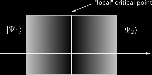
16 Symmetry breaking paradigm ˆ ˆ : 16 / 59

17 ˆ ( ) 1 2π d 2 k B(k) = ( ) = ( ) ˆ C.f. σ xy 1 : ( ) = 1 4π 2 17 / 59

18 ˆ ( ) ˆ = ˆ = 18 / 59

19 ˆ ˆ 19 / 59

20 ˆ gapless 20 / 59

21 ˆ U(1) ˆ ( ) ( ) / 59

22 J ( e) ( d d k ( τ ħ E k f 0 ) ε ħ k } {{ } dynamical part e + f 0 E ħ B ) }{{} topological part ˆ ( ) ˆ (e.g., ) ˆ (No dynamics, no Joule heating) ˆ : ˆ ˆ ˆ ˆ etc. 22 / 59

23 Topological phases beyond the quantum Hall eect? ˆ 2 ˆ ˆ 23 / 59

24 Topological systems. Related concepts / (SPT ). 24 / 59

25 ˆ ˆ ˆ ˆ ˆ ˆ interplay: ˆ (Symmetry-Protected Topological phases; SPT ) ˆ (Symmetry-Enriched Topological phases;set ) 25 / 59

26 (SPT ) ˆ SPT ˆ SPT 26 / 59

27 ˆ ˆ Symmetry-breaking paradigm ˆ 27 / 59

28 Phases of condensed matter Spontaneous symmetry breaking Phases of matter No spontaneous symmetry breaking Ordered phases Quantum disordered phases Gapless Gapped Gapless Gapped Continuous symmetry-broken phases Discrete symmetry-broken phases Quantum critical disordered phases and critical points Gapped quantum disordered phases No topological order Topological order Other phases Symmetry breaking coexists with topological order... Trivial phases Short-range entangled states (a.k.a "invertible" states) Symmetry Topologically ordered phases Long-range entangled states Symmetry Symmetry protected topological phases (SPT phases) Symmetry enriched topological phases (SET phases) 28 / 59

29 ˆ H = J i S i S i+1, J > 0 ˆ Gapped, unique ground state, no SSB = ˆ SPT 29 / 59

30 ˆ 1/2 ˆ (( 1) ) ˆ C.f. RVB 30 / 59

31 ˆ Ψ = 1 2 [ ] ˆ ρ = Ψ Ψ = 1 [ ] 2 ρ T 2 = 1 [ ] 2 ˆ ˆ Spec(ρ T1 ) = {1/2, 1/2, 1/2, 1/2}. ˆ C.f. ρ = 1 2 [ ] = ρt 2 31 / 59

32 ˆ : for the density matrix ρ A1 A 2, e (1) i e (2) j ρ T 2 A 1 A 2 e (1) k e(2) l = e (1) i e (2) where e (1,2) i is the basis of H A1,A 2. ˆ = H = H T l ρ A1 A 2 e (1) k e(2) j ˆ detect Entanglement negativity and logarithmic negativity 1 2 (Tr ρt 2 A 1), E A = log Tr ρ T 2 A [Peres (96), Horodecki-Horodecki-Horodecki (96), Vidal-Werner (02), Plenio (05)...] 32 / 59

33 ˆ Partial transpose can be used to construct/dene topological invariants of bosonic topological phases [Pollmann-Turner] ˆ Start from the reduced density matrix for the interval I, ρ I := Tr Ī Ψ Ψ. ˆ I consists of two adjacent intervals, I = I 1 I 2. ˆ Consider partial time-reversal acting only for I 1 ; ρ I ρ T1 I. ˆ Partial time reversal partial transpose. 33 / 59

ˆ The invariant is given by the phase of: Z =

= A s 1 i 1 i 2 A s 2 i 2 i 3 A s 3 i 3 i 4 s

34 ˆ The invariant is given by the phase of: Z = Tr[ρ I ρ T1 I ]. C.f. Negativity: Tr ρ T 1 I ˆ Matrix product state representation: ˆ Wave function; Ψ(s 1, s 2, ) = A s 1 i 1 i 2 A s 2 i 2 i 3 A s 3 i 3 i 4 s a =, {i n =1, } ˆ Topological invariant: : Z = Tr[ρ I ρ T 1 I ] 34 / 59

35 ˆ The invariant "simulates" the path integral on real projective plane RP 2 : [Shiozaki-Ryu (16)] = = = = 35 / 59

36 ˆ ˆ = ( ) + BdG ( ) ˆ Bogoliubov-de Genne : H = 1 ( Ψ ξ H Ψ, H = 2 ξ T where Ψ = (ψ, ψ, ψ, ψ ) T ) ˆ BdG " " 36 / 59

37 ˆ ˆ = ( ) + BdG ( ) ˆ Bogoliubov-de Genne : H = 1 ( Ψ ξ H Ψ, H = 2 ξ T where Ψ = (ψ, ψ, ψ, ψ ) T ) ˆ BdG " " 37 / 59

38 ˆ ˆ = ( ) + BdG ( ) ˆ Bogoliubov-de Genne : H = 1 ( Ψ ξ H Ψ, H = 2 ξ T where Ψ = (ψ, ψ, ψ, ψ ) T ) ˆ BdG " " 38 / 59

39 ˆ ˆ = ( ) + BdG ( ) ˆ Bogoliubov-de Genne : H = 1 ( Ψ ξ H Ψ, H = 2 ξ T where Ψ = (ψ, ψ, ψ, ψ ) T ) ˆ BdG " " 39 / 59

40 ˆ ( = t ) H = [ ] tc j c j+1 + c j+1c j + h.c. µ j j c j c j 40 / 59

41 ˆ ˆ 2 t µ ˆ Z 2 [ π ] exp i dk A x(k) = ±1 π (A x (k) = i u(k) / k u(k) ) 41 / 59

42 ˆ ˆ The end state is a Majorana fermion. γ = γ 42 / 59

43 ˆ ˆ The end state is a Majorana fermion. γ = γ 43 / 59

44 ˆ γ dr ( u(r)c(r) + u (r)c (r) ) ˆ γ = γ ˆ complex fermion f = γ 1 + iγ 2 ˆ ˆ 44 / 59

45 ˆ γ dr ( u(r)c(r) + u (r)c (r) ) ˆ γ = γ ˆ complex fermion f = γ 1 + iγ 2 ˆ ˆ 45 / 59

46 ˆ γ dr ( u(r)c(r) + u (r)c (r) ) ˆ γ = γ ˆ complex fermion f = γ 1 + iγ 2 ˆ ˆ 46 / 59

47 ˆ γ dr ( u(r)c(r) + u (r)c (r) ) ˆ γ = γ ˆ complex fermion f = γ 1 + iγ 2 ˆ ˆ 47 / 59

48 ˆ γ dr ( u(r)c(r) + u (r)c (r) ) ˆ γ = γ ˆ complex fermion f = γ 1 + iγ 2 ˆ ˆ 48 / 59

49 ˆ c x = c L x + ic R x, c x = c L x ic R x. 49 / 59

50 ˆ Proximitized spin-orbit quantum wire [Mourik et al (12)], ˆ Magnetic adatomes on the surface of an s-wave superconductor [Nadj-Perge et al (14)] 50 / 59

51 ˆ ˆ ˆ I tell my students that 2017 is the year of braiding. Kouwenhoven@Microsoft and Delft, Nature (05 January 2017) 51 / 59

52 ˆ Can partial transpose/negativity can capture fermionic entanglement? ˆ An example in 1+1 dimensions: the Kitaev chain (with t = ) H = [ ] tf xf x+1 + f x+1f x + h.c. µ f xf x x x 52 / 59

53 ˆ Consider log negativity E for two adjacent intervals of equal length. (L = 4l = 8) ˆ Vertical axis: µ/t ranging from 0 to 6. ˆ (Blue circles and Red corsses) is computed by Jordan-Wigner + bosonic partial transpose ˆ Log negativity fails to capture Majorana dimers. 53 / 59

54 Topological insight into partial transpose in topological phases ˆ ˆ 54 / 59

55 Partial transpose for fermions our denition [Shiozaki-Shapourian-SR (16)] ˆ Expand the density matrix in terms of Majorana fermions: ˆ ρ A = w κ,τ c κ 1 m 1 c κ 2k m 2k κ,τ }{{} H 1 τ c 1 n 1 c τ 2l n }{{ 2l } H 2 ρ T 1 A = κ,τ w κ,τ R(c κ 1 m 1 c κ 2k m 2k ) c τ 1 n 1 c τ 2l n 2l = κ,τ w κ,τ i κ c κ 1 m 1 c κ 2k m 2k c τ 1 n 1 c τ 2l n 2l where R satises: R(c) = ic, R(M 1 M 2 ) = R(M 1 )R(M 2 ) ˆ Simple check: (ρ T 1 A )T 2 = ρ T A, (ρ T A) T = ρ A, (ρ 1 A ρ n A) T 1 = (ρ 1 A) T 1 (ρ n A) T 1 55 / 59

56 [Shiozaki-Shapourian-SR (16)] ˆ (Blue circles and Red crosses): Old (bosonic) denition ˆ (Green triangles and Orange triangles) Our denition; 56 / 59

57 ˆ : Z = Tr (ρ I ρ T1 I ); ˆ ˆ Z [Fidkowski-Kitaev(10)] 57 / 59

58 ˆ Fermionic partial transpose ˆ Fermionic partial transpose (C.f. TKNN Kane-Mele ) 58 / 59

59 Outlook ˆ ˆ Many future applications, in particular, in numerics. ˆ NbSe 3 Möbius strip [Ningyuan-Owens-Sommer-Schuster-Simon (13)] 59 / 59

Êª¼Á¤Î¥È¥Ý¥í¥¸¥«¥ë¸½¾Ý (2016Ç¯¥Î¡¼¥Ù¥ë¾Þ¤Ë´ØÏ¢¤·¤Æ) (2016 ) Dept. of Phys., Kyushu Univ. 2017 8 10 1 / 59 2016 Figure: D.J.Thouless F D.M.Haldane J.M.Kosterlitz TOPOLOGICAL PHASE TRANSITIONS AND TOPOLOGICAL PHASES OF MATTER 2 / 59 ( ) ( ) (Dirac, t Hooft-Polyakov)