4 19

Size: px

Start display at page:

Download "4 19"

たつやおおはし
5 years ago
Views:

1 I /

2 4 19

4 :

5 : f(e, J), f(e) Phase mixing Landau Damping, violent relaxation

7 : 2 2

8 :

10 ( )

13 ( )

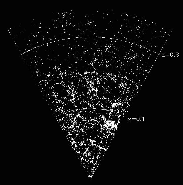
14 ( ) SDSS

15 ( ) (< 10 4 ) M5, ω Cen, 47 Tuc 10 6 ( )

17 Arches Cluster 30pc > 10 4 M 1pc 4 : Nagata et al (1995)

18 ( ) ( )

19 Genzel et al 2003 K-band shift-and-add image SgrA ( )

20 ( ) Genzel et al M ( ) 0.5 (S1, S2, S )

21 Eisenhauer et al (10M )

24 ? m i d 2 x i dt 2 = j i f ij (1) x i m i i f ij j i f ij G f ij = Gm i m j x j x i x j x i 3, (2)

25 ( ) 2 ( ) 3

26 YES NO

27 : +9(8) ( ) 0 ( )

28 ( ) : 3 0.1%

29 19

30 20 20

31 2

32 ( )

33 (1 )

34 3 3 (2 )

35 3 3

36 3 2,3 Sun L4 L5 Jupiter

37 2006 IAU Genearal Assembly ( )

38 II 10 Figure-8 Solution Edinburgh Douglas Heggie

39 Figure-8 solution 3 (0.005% )

41 1987 2

42 e 2 8.5

43 45 2

44 100

46 : : 1000 ( )

47 : : 10 7 : : 10 5 ( )

50 d 2 x i dt 2 = j i Gm j x j x i x j x i 3, (3) (1 ) f(x, v, t) :( )

51 ( ) f f + v f Φ = 0, (4) t v f:6 Φ :, 2 Φ = 4πGρ. (5) G ρ ρ = m dvf, (6) m f

52 BBGKY : f t + v f Φ f v 6 Df/Dt = 0:

53 1 w = (x, v, t) Φ = Φ(x, t) ẇ = (ẋ, v) = (v, Φ) (7) f t + 6 (fẇ i ) = 0, (8) i=1 w i 2 w 6 i=1 ẇ i w i = 3 i=1 v i + v i x i v i = 3 i=1 v i Φ = 0 (9) x i

54 2 w f t + v f Φ f v f:6 = 0, (10) Φ :, 2 Φ = 4πGρ. (11) G ρ ρ = m dvf, (12)

55 = f Φ = Φ f Φ f 0

56 f (f log f )

57 :

58 : ( ) : ( )

59 :

60 ( ) ( )

61 : 2 : 2 :

62 2 ( ) : : : ( )

63 : =

64 ( ) ( )

65 : :

66 =

67 ( ) : N 1/N ( ) N

68 N 1/ N 1 1/ N N

69 N/ log N

71 : Jeans

72 Φ x, v I d I(x, v) = 0, (13) dt v I Φ I v = 0 (14)

73 : : 1 2 v2 + Φ r L = r v

74 : Φ f I 1, I 2,..., I m f = f(i 1, I 2,..., I m )

75 : f OK ( ) f I k 0 5

76 3 4 :

78 f(e, J) f E J f J f(e, J) 1 d r 2 dr r 2dΦ = 4πG dr f 1 2 v2 + Φ, r v dv, (15) f(e, J)

79 f(e) J < v 2 e >= 1 ρ v 2 e f(v2 + Φ)dv (16) f v v e

80 f(e) ( ) Ψ = Φ + Φ 0, E = E + Φ 0 = Ψ v 2 /2 (17) Φ 0 E > 0 f > 0, E f = 0 v 1 d r 2 dr r 2dΨ dr = 16π 2 G 2Ψ 0 f(ψ 1 2 v2 )v 2 dv = 16π 2 G Ψ 0 f(e) 2(Ψ E)dE. (18) f Ψ

81 Hernquist

82 E F E f(e) = n 3/2 (E > 0) (19) 0 otherwize Ψ ρ = c n Ψ n (Ψ > 0) (20) c n n > 1/2 ρ 1 d r 2 dr r 2dΨ + 4πGc n Ψ n = 0 (21) dr

83 Lane-Emden 1 d r 2 dr r 2dΨ + 4πGc n Ψ n = 0 (22) dr 1 d s 2 ds s 2dψ ds Lane-Emden + ψ n = 0 (23) Lane-Emden

84 n Lane-Emden n = 5 1 φ = (24) s2 c 5 φ 5 r = 0 r 1/r 3 self-consistent

85 Lane-Emden P ρ 1+1/n (25) : ( ) :

86 Hernquist Model 1990 (Hernquist, L., 1990, ApJ 356, 359) Φ = 1 r + a ρ = C (26) a r(r + a) 3 (27)

87 Hernquist Model r 1/4 Hernquist Model r 1/4 ( ) r 1/4 1/4

88 Hernquist Hernquist : ( ) Jaffe Dehnen Tremaine η 3 ( ) Navarro-Frenk-White (NFW) Moore

89 Dehnen Model ρ = C γ = 1: Hernquist model γ = 2: Jaffe model a r γ (r + a) 3 γ (28)

90 NFW Moore NFW (NFW1996) ρ = C a r(r + a) 2 (29) Moore (Moore et al 1999) a ρ = C r 1.5 (r a 1.5 ) (30)

91 f(e) = ρ 1 (2πσ 2 ) 3/2eE/σ2 = ρ 1 exp (2πσ 2 ) 3/2 Ψ v 2 /2 σ 2 (31)

92 ( ) 2 e x2 dx = 1 (32) π 0 ρ = ρ 1 e Ψ/σ2 (33) 1 d r 2dΨ r 2 = 4πGρ (34) dr dr 1 r 2 d dr r 2d log ρ = 4πGσ 2 ρ (35) dr

93 ( 2) ρ = (36) 2πGr 2 (singular isothermal sphere) self consistent : M r r flat rotation curve : ρ 1/r 2 ( ) r singular isothermal σ2

94 dp dr = ρgm r (37) r 2 P = k BT m ρ (38) P M r C d dr r 2d log ρ = 4πGρr 2 (39) dr

95 stellar system stellar system

96 King Model 0 :

97 f(e) = ρ 1 (2πσ 2 ) 3/2eE/σ2 = ρ 1 exp (2πσ 2 ) 3/2 Ψ v 2 /2 σ 2 (40) : (E ) 0

98 Lowered Maxwellian f(e) = ρ 1 (2πσ 2 ) 3/2 (e E/σ2 1) (E > 0) 0 (E 0) (41) E = 0 f = 0 1

99 ρ = 4πρ 1 (2πσ 2 ) 3/2 = ρ 1 2Ψ 0 e Ψ/σ2 erf Ψ σ exp Ψ v 2 /2 1 v 2 dv 4Ψ πσ 2 σ Ψ 3σ 2 (42) erf 1 erf(z) = 2 π z 0 e t2 dt. (43)

100 dψ/dr = 0 Ψ 0

101 Ψ 0 1, 3, 6, 9, 12 r 0 r 0 = 9σ 2 (44) 4πGρ 0

102 ( ) r t ρ 0 ( Ψ 0 ) : King model tidal radius King Model c = log(r t /r 0 ) concentration parameter Ψ 0

103 :

104 X Einstein IPC Hydra A (David et al. ApJ 1990, 356, 32)

105 Chandra

106

107 ρ g ρ s d dr ρ s r 2d log ρ g = 4πGm dr k B T ρ sr 2 (45) ρ g ρ g = Cρ s (46)

108 T g T s T g /T s = 1/β d dr r 2d log ρ g = β[ (45) ] (47) dr ρ g = Cρ β s (48) β

109 : :

110 ρ = ρ 0 [1 + (r/r c ) 2 ] 3/2 (49) β Sarazin X-ray emissions from clusters of galaxies 5.5 β (48) ρ s ρ s r < 2.5r c

111 β 1 ρ = ρ 0 [1 + (r/r c ) 2 ] 3/2 (50) ρ = ρ 0 [1 + (r/r c ) 2 ] 3β/2 (51) X X = 2 I(r) = 2 0 ρ( r 2 + z 2 ) 2 dz (52) I(r) = C[1 + (r/r c ) 2 ] 3β+1/2 (53)

112 β : (Jones and Forman 1984) Hydra A

113 β 2 Ikebe et al. 1997, ApJ 481, 660

114 β excess Cooling flow β β β 2

115 Cooling flow cluster β β isothermal

116

117

118

119 ρ f f(e) f(e) ρ(r) = 4π Ψ 0 f(e) 2(Ψ E)dE. (54) Ψ r ρ Ψ Ψ 1 dρ 8π dψ = Ψ 0 f(e)de Ψ E (55)

120 ρ f 1 dρ 8π dψ = Ψ 0 f(e)de Ψ E (56) Abel f(e) = 1 8π 2 f(e) = 1 8π 2 E 0 d 2 ρ dψ 2 d de E 0 dρ dψ dψ + 1 E Ψ E dψ E Ψ (57) dρ dψ Ψ=0 (58)

121 :Jaffe model Jaffe model ρ = r 4 J r 2 (r + r J ) 2, Ψ = ln r r + r J r Ψ ρ (59) ρ = (e Ψ/2 e Ψ/2 ) 4 (60) 58 x = E Ψ E = Er j /GM f(e) = M 2π 3 (GMr J ) 3/2[F ( 2E) 2F ( E) 2F + ( E) + F + ( 2E)] (61)

122 F ± = e x2 x 0 e±x 2 dx (62)

123 Jeans Equations f t + v f Φ f v = 0, (63) 3 0

124 ( ) 2 ν = fd 3 v; v i = 1 ν fvi d 3 v (64) ν t + (ν v i) x i = 0 (65)

125 1 Collisionless Boltzman v j fvj d 3 v + f v i v j d 3 v Φ f vj d 3 v = 0, (66) t x i x i v i i v j f 1 (ν v j ) vj f v i d 3 v = t + (νv iv j ) x i v j v i fd 3 v = δ ij ν (67) + ν Φ x j = 0 (68)

126 v i v j v i v j ν/ t ν v j t v (ν v i ) j + (νv iv j ) x i x i + ν Φ x j = 0 (69) σ 2 ij = (v i v i )(v j v j ) (70)

127 Jeans ν v j t + ν v v j i = ν Φ (νσ2 ij ) (71) x i x j x i Lagrange stress tensor σij 2 stress tensor σ 2 I I

128 M/L Jeans equation d(νv 2 r ) dr + ν r [ 2v 2 r ( v 2 θ + v2 φ)] = ν dφ dr (72) 1 d(νvr 2) ν dr M(r) = rv2 r G = dφ dr d ln ν d ln r + d ln v2 r d ln r (73) (74)

129 M/L M(r) = rv2 r G d ln ν d ln r + d ln v2 r d ln r (75) ν luminosity

130 M/L M/L M/L

131 68 ν ρ x k xk (ρ v j ) t d 3 x = x k (ρv i v j ) x i d 3 x ρx k Φ x j d 3 x (76) xk (ρv i v j ) x i d 3 x = δ ki ρv i v j d 3 x = 2K kj (77) K W

132 ( ) σ 2 K jk = T jk Π jk (78) T jk = 1 2 ρ vj v k d 3 x, Π jk = ρσ 2 jk d3 x, (79) j, k k, j 1 d 2 dt ρ(xk v j + x j v k )d 3 x = 2T jk + Π jk + W jk (80)

133 ( 2) I jk = ρx j x k d 3 x (81) di jk dt = ρ(x k v j + x j v k )d 3 x (82) 1 d 2 I jk = 2T 2 dt 2 jk + Π jk + W jk (83)

134 I 0 T, Π K 2 W Φ W = ρ k x k Φ x k d 3 x = ρ(x)ρ(x ) k x k (x k x k ) x x 3 d 3 xd 3 x x x (84) W = 1 2 ρ(x)ρ(x ) (x k x k )2 k x x 3 d3 xd 3 x = 1 2 ρφd 3 x (85) W

135 ( ) 2K + W = 0 (86) E E = K + W E = K = W/2 (87)

136 King model K = E

137 z W xx = W yy ; W ij = 0 (i j) (88) 2T xx + Π xx + W xx = 0; 2T zz + Π zz + W zz = 0 (89) 2 2 2T xx + Π xx 2T zz + Π zz = W xx W zz (90)

138 T zz = 0 2T xx = 1 2 ρv 2 φ d3 x = 1 2 Mv2 0 (91) v 0 Π xx = Mσ 2 0 (92) (r.m.s) z x δ Π zz = (1 δ)πxx (93)

139 2 v 2 0 σ 2 0 = 2(1 δ) W xx W zz 2 (94) W xx /W zz : ρ = ρ(m); m 2 = a i=1 x 2 i a 2 i (95) W ii /W jj a ρ(m)

140 3 Binney and Tremaine( BT) δ ε1 b/a v 0 σ 0

141 4 BT : : ε v 0 σ 0 : δ = 0

142 5 δ = 0

143 6 Okumura et al. (1991, PASJ 43, 781)

144 7 2 4 r p /r h = 2.6 v 0 /σ 0

145 CBE

146 ρ + (ρv) = 0 (96) t v t + (v )v = 1 p Φ (97) ρ 2 Φ = 4πGρ (98)

147 ρ, p, v, Φ ρ = ρ 0 + ρ v s ρ 1 t + (ρ 0v 1 ) + (ρ 1 v 0 ) = 0 (99) v 1 t + (v 0 )v 1 + (v 1 )v 0 = ρ 1 p ρ p 1 Φ 1 0 ρ 0 (100) 2 Φ 1 = 4πGρ 1 (101) dp p 1 = ρ 1 = v 2 s dρ ρ 1 (102)

148 0 2 ρ 1 t + ρ 1 (ρ 0 v 1 ) = 0 (103) v 1 t = 1 p 1 Φ 1 ρ 0 (104) 2 ρ 1 2 ρ 1 t 2 v2 s 2 ρ 1 4πGρ 0 ρ 1 = 0 (105)

149 2 ρ 1 t 2 v2 s 2 ρ 1 4πGρ 0 ρ 1 = 0 (106) 2

150 ρ 1 = Ce i(k x ωt) (107) ω 2 = v 2 s k2 4πGρ 0 (108)

151 ( ) k 2 J = 4πGρ 0 v 2 s (109) k > k J ω k = k J ω = 0 k < k J ω

152 ( 2) 1/k J

153 f f + v f Φ = 0, (110) t v f 6 Φ 2 Φ = 4πGρ. (111) G ρ ρ = m dvf, (112)

154 f 0 + f 1 Φ 0 + Φ 1 0 f 1 t + v f 1 Φ 0 f 1 v Φ 1 f 0 v = 0, (113) 2 Φ 1 = 4πG f 1 dv. (114)

155 Jeans f 0 Φ 0 f 1 t + v f 1 Φ 1 f 0 = 0, (115) v f 1 = f a (v) exp[i(k x ωt)] (116) Φ 1 = Φ a exp[i(k x ωt)] (117)

156 ( ω + v k)f a (v) Φ a k f 0 v = 0 (118) k 2 Φ a = 4πG f a dv (119) f a Φ a 1 + 4πG k 2 k f 0 v dv = 0 (120) k v ω f 0 k ω

157 1 + 4πG k 2 k f 0 v dv = 0 (121) k v ω k v ω = 0 0

158 ( ) x 1 + 4πG k 2 k f 0 v x dv = 0 (122) kv x ω ω = 0 k 2 J = 4πG f 0 v x v x dv (123) f 0 v x = 0 ω = 0 k J

159 f 0 f 0 (v) = ρ 0 exp (2πσ 2 ) 3/2 v 2 /2 (124) σ 2 e v2 2σ 2 dv = 2πσ 2 (125) k 2 J = 4πGρ 0 σ 2 (126)

160 ω = iγ πGρ 0 kσ 3 vx e v2 x /2σ2 kv x iγ dv x = 0 (127) v x (kv x + iγ)e v2 x /2σ2 k 2 v 2 x + γ2 dv x = 0 (128)

161 ( ) 0 x 2 e x2 x 2 + β 2dx = 1 1 π 2 2 πβeβ2 [1 erf(β)] (129) k 2 = k 2 J πγ 1 exp 2kσ γ 2 2k 2 σ 2 1 erf γ 2kσ (130) k ω (γ) k < k J γ k = k J k = 0

162 ( 2)

163 van Kampen mode :

164 Phase Mixing : 1 (overdensity)

165 Phase Mixing ( ) v v v x x x singular van Kampen mode phase mixing

166 S = f ln fdxdv (131) g(x, v; h) g(x, v; h)dxdv = 1 (132) lim h 0 fg(x0 x, v 0 v; h)dxdv = f(x 0, v 0 ) (133) δ

167 ˆf h ˆf h = fg(x x 1, v v 1 ; h)dx 1 dv 1 (134) Ŝ = ˆf ln ˆfdxdv (135)

168 Ŝ

169 Wave-particle interaction /

170 Wave-particle interaction ( ) v w v p v p v w

171 Wave-particle interaction ( 2)

172 Dynamical Friction 0 OK

173 Dynamical Friction ( )

174 Dynamical Friction ( 2) = dynamical friction 3

175 Dynamical Friction ( 3) Dynamical Friction

176 Violent relaxation Phase mixing phase mixing Phase mixing

177 r 1/4 Hernquist Profile

178 Violent Relaxation Lynden-Bell (1967) violent relaxation

179 Violent Relaxation ( ) Lynden-Bell

180 Violent Relaxation ( ) phase mixing Lynden-Bell Lynden-Bell Maxwell-Boltzman f Lynden-Bell

181 violent relaxation

182 van Albada (1982, MNRAS 201, 939) : 1982 N = 5000 :

183 N(E) N(E) : N(E)dE = dn

184 : violent relaxation

185

186

187 N(E)

188 Lynden-Bell violent relaxation

189 Violent relaxation violent relaxation 2

190 N(E) Lynden-Bell IAU Symposium 127 Structure and Synamics of Elliptical Galaxies Scott Tremaine (Conference Summary) W. Jaffe (Poster) Jaffe

191 N(E) (2) 0 0

192 N(E) (2) : 0

193 0 phase volume 0 N(E) 0 van Albada N(E) E = 0 r N(E) = N 0 + N 0 E N 0 > 0

194 N(E) N(E) Φ = M/r (136) E = M 2r (137)

195 dm = 4πr 2 ρdr = N(E)dE (138) 137 de dr = M 2r 2 (139) ρ = MN(E) 8πr 4 (140) 4 4

196 : Jaffe (1987)

197 E (r, r+ dr) P (E, r)dr 4πr 2 ρ = 0 E r P (E, r)n(e)de (141) E r r M/r P (E, r) P (E, r) = P 0 (r/r E )/r E (142) r E = M/E

198 x = re/m ρ = M 0 4πr P 4 1 0(x)xN(Mx/r)dx (143) r radial orbit J N(E, J) J OK

199 N(E) N(E) E 0 ρ r 4 Hernquist model Jaffe model ρ r 4

200 10 Navarro ApJ 1997, 490, 493) CDM CDM ρ 1 r (1 + r ) 2 (144) NFW

201 Navarro CDM Fukushige and Makino (ApJ 1997, 477 L9) Moore et al. (ApJ 1998, 499, 5L ) Navarro 1.5 Navarro 1 Fukushige Moore 100

202 2 half mass radius 0 1.5

A 99% MS-Free Presentation

A 99% MS-Free Presentation 2 Galactic Dynamics (Binney & Tremaine 1987, 2008) Dynamics of Galaxies (Bertin 2000) Dynamical Evolution of Globular Clusters (Spitzer 1987) The Gravitational Million-Body Problem