, 3, STUDY ON IMPORTANCE OF OPTIMIZED GRID STRUCTURE IN GENERAL COORDINATE SYSTEM 1 2 Hiroyasu YASUDA and Tsuyoshi HOSHINO

Size: px

Start display at page:

Download ", 3, STUDY ON IMPORTANCE OF OPTIMIZED GRID STRUCTURE IN GENERAL COORDINATE SYSTEM 1 2 Hiroyasu YASUDA and Tsuyoshi HOSHINO"

しょうじはまもり
4 years ago
Views:

1 , 3, STUDY ON IMPORTANCE OF OPTIMIZED GRID STRUCTURE IN GENERAL COORDINATE SYSTEM 1 2 Hiroyasu YASUDA and Tsuyoshi HOSHINO Numerical computation of river flows have been employed the general coordinate system to adjust a river plane form. An adjustment flexibility of the coordinate system is better but it is difficult to generate a grid system in order to compute stably because grid system is not determined uniquely. This study develops a new boundary fitting method introducing the hierarchical quad-tree grid system for computation of confluence and bifurcation in natural rivers. The numerical model with the quad-tree grid system apply to compute flow pattern in experiment flume and in natural river with bifurcation and confluence, the computed results agree with measured result of the flume and natural river well. Key Words: truncation error, metric, general curvilinear coordinate system, numerical grid generation 1. Taylor 0 Thompson 1) Thompson 49

2 2. 1 x ξ, y η x ξξ, y ηη x η, y ξ x ηη, y ξξ x ξη, y ξη -1 x ξ, y η f x = f ξ x ξ (1) f 1 x ξ 1 (i, j) f x = f i+1 f i 1 x i+1 x i 1 (2) Taylor f x f xx f xx f f i+1, f i 1 Taylor (2) T = 1 2 x ξξf xx 1 6 x2 ξf xxx + O( ξ 4 ) (3) f x = 1 J [y ηf ξ y ξ f η ] (4) f y = 1 J [ x ηf ξ + x ξ f η ] (5) x, y ξ, η x = x(ξ, η), y = y(ξ, η) ξ = ξ(x, y), η = η(x, y) J x ξ y η x η y ξ f η, f ξ Taylor (4) (5) T x = 1 2J [(y ξx η x ηη y η x ξ x ξξ ) f xx + (y ξ y η y ηη y η y ξ y ξξ ) f yy + {y ξ (x η y ηη + y η x ηη ) y η (x ξ y ξξ + y ξ x ξξ )} f xy ] + O( ξ 3 ) (6) T y = 1 2J [( x ξx η x ηη + x η x ξ x ξξ ) f xx + ( x ξ y η y ηη + x η y ξ y ξξ ) f yy + { x ξ (x η y ηη + y η x ηη ) +x η (x ξ y ξξ + y ξ x ξξ )} f xy ] + O( ξ 3 ) (7) 1) T x, T y (4) (5) 10 1 x ξ, y η 0 x ξξ, y ηη (i, j) x ξξ = x i+1,j 2x i,j + x i 1,j (8) 3. (1) Thompson 2) αx ξξ 2βx ξη + γx ηη = 0 (9) αy ξξ 2βy ξη + γy ηη = 0 (10) α = x 2 η + y 2 η (11) 50

3 β = x ξ x η + y ξ y η (12) γ = x 2 ξ + y 2 ξ (13) 2 x y (9) (10) (uh) t (vh) t + (hu2 ) x + (huv) = hg H y x τ x ρ +Dx (16) + (huv) + (hv2 ) = hg H x y y τ y ρ +Dy (17) H t + (uh) + (vh) = 0 (18) x y τ x ρ = C du u 2 + v 2 (19) τ y ρ = C dv u 2 + v 2 (20) (2) 1 x ξ, y η 0 (6) T x = 1 2 x ξξf xx (y ηηf yy x ξξ f xy ) cot θ (14) θ 45 L = n l (15) L l n (9) (10) 4. iric 2 Nays2D D x = ( ) (uh) ν t + ( ) (uh) ν t x x y y D y = ( ) (vh) ν t + ( ) (vh) ν t x x y y (21) (22) (2)(3) (x, y) 2 (4) u x v y h H g ρ τ x x τ y y ν t 5. (1) (a) (b) (c) (a) (d) (e) (a) 2 (e) (e) 51

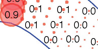
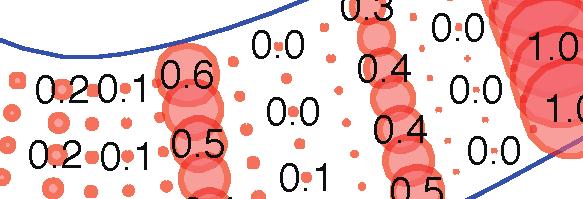
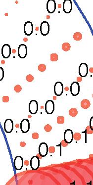
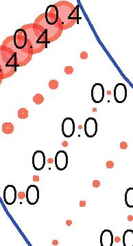
4 i) 格子構成 ii) メトリックスの打切り誤差 iii) 累積水位変動量 (a) 格子構成 1 測量測線に基づく格子構成 (b) 格子構成 1-0 経験に基づく手動による最適化 (c) 格子構成 1-1 楕円型方程式による最適化 (d) 格子構成 1-2 楕円型方程式による最適化と境界値の等配分 (e) 格子構成 2 測量測線に基づく格子構成縦断方向 2 倍図-1 格子構成メトリックスの打切り誤差解の安定性

5 (2) a) T x, T y f xx, f yy, f xy T x = 1 2J [(y ξx η x ηη y η x ξ x ξξ ) + (y ξ y η y ηη y η y ξ y ξξ ) + {y ξ (x η y ηη + y η x ηη ) y η (x ξ y ξξ + y ξ x ξξ )} ] (23) T y = 1 2J [( x ξx η x ηη + x η x ξ x ξξ ) + ( x ξ y η y ηη + x η y ξ y ξξ ) + { x ξ (x η y ηη + y η x ηη ) +x η (x ξ y ξξ + y ξ x ξξ )} ] (24) 5 1 T xy T xy T xy (i, j) = 1 S (T x(i, j) + T y (i, j)) (25) S x, y 1(a) (8) (b) (a) (c) (d) (a) (c) (a) (a) (d) (e) (a) 5 b) H(i, j) δh(i, j) = dt (26) H 0 (i, j) H 0 1(b) 1(a) (e) (b) (c) (d) (a) (e) 1 (e) (a) (25) 6. (A)( ) (B)( ) 53

6 1) Joe F. Thompson, Z.U.A. Warsi and C. Wayne Mastin, Numerical Grid Generation Foundations and Applications, 2) Thompson, J. F.; Mastin, C. W.; Thames, F. C., Automatic numerical generation of body-fitted curvilinear coordinate system for field containing any number of arbitrary two-dimensional bodies, doi:1016/ (74) , J Compt Phys, pp ,

, COMPUTATION OF SHALLOW WATER EQUATION WITH HIERARCHICAL QUADTREE GRID SYSTEM 1 2 Hiroyasu YASUDA and Tsuyoshi HOSHINO

, COMPUTATION OF SHALLOW WATER EQUATION WITH HIERARCHICAL QUADTREE GRID SYSTEM 1 2 Hiroyasu YASUDA and Tsuyoshi HOSHINO , 2 11 8 COMPUTATION OF SHALLOW WATER EQUATION WITH HIERARCHICAL QUADTREE GRID SYSTEM 1 2 Hiroyasu YASUDA and Tsuyoshi HOSHINO 1 9-2181 2 8 2 9-2181 2 8 Numerical computation of river flows have been employed