Einmahl and Magnus (2007) Records in athretics through extreme-value theory. 04:35

Size: px

Start display at page:

Download "Einmahl and Magnus (2007) Records in athretics through extreme-value theory. 04:35"

ぜんぺいみしま
7 years ago
Views:

1 ( ) r-taka@maritime.kobe-u.ac.jp

2 Einmahl and Magnus (2007) Records in athretics through extreme-value theory. 04:35

3 Age Castillo, Hadi, Balakrishnan and Sarabia (2004) p The yearly oldest ages at death in Sweden during the period from 1905 to 1958 for women

4 (m/s)

5 Kumamoto Max. Daily Rainfall Year (0.1mm)

6 Nara Daily Rainfall (0.1mm) Day Nara Daily Rainfall (0.1mm) Day (0.1mm)

7 Daily Maximum Temperature Kyoto ( 0.1 C)

9 Coles A. B.

10 (block maximum) Fréchet Fisher and Tippett von Mises Gnedenko

11 1960 Geffroy Tiago de Oliveira Sibuya Gumbel (1958)

12 Peaks Over Threshold (POT) (threshold exceedances Balkema and de Haan (1974) Pickands (1975) r Weissman (1978) Smith (1986) Tawn (1988)

13 X 1, X 2,..., X n,... F (x) = P (X i x), i = 1, 2,... X 1, X 2,..., X n X (1:n) X (2:n)... X (n:n) Z n = X (n:n) = max { X 1, X 2,..., X n } = max 1 i n X i

14 n Z n F x + Z n x + = sup{x : F (x) < 1}, n. Z n a n > 0, b n R (n = 1, 2,...) G(x) Z P ( Zn b n Z n b n a n d Z, n. a n ) x P (Z x) = G(x). G (extreme value distribution) F G (maximum domain of attraction) F MDA(G) (a n, b n )

15 (1) G(x) (2) F MDA(G) F (3) a n b n W n = min 1 i n X i W n = min { } { } X 1, X 2,..., X n = max X1, X 2,..., X n W G W (x) = 1 G( x)

16 P ( Zn b n a n ) x = P (Z n a n x + b n ) = P ( max 1 i n X i a n x + b n ) = P (X i a n x + b n, i = 1, 2,..., n) = n i=1 P (X i a n x + b n ) = F n (a n x + b n ).

17 lim n F n (a n x + b n ) = G(x), x R. a n x + b n x + = sup{x : F (x) < 1} y = a n x + b n ( ) P (Z n y) = F n y bn (y) G. a n Xi = µ + σx i i = 1, 2,..., n µ R σ > 0 = Z n = max 1 i n X i = µ + σ max 1 i n X i = µ + σz n.

18 0 < G(x) < 1 lim n F n (a n x + b n ) = G(x) lim n[1 F (a n n x + b n )] = log G(x). { F n (a n x+b n ) = 1 + n[1 F (a nx + b n )] n } n { } exp lim n[1 F (a n n x+b n )] ( x n x, n = lim 1 + x ) n n = e x. n n

19 Block Maximum from Exp(1) Block Maximum from N(0, 1) maximum Block Maximum from Par(2) maximum Block Maximum from U(0, 1) maximum maximum

0 maximum Block Maximum from U(0, 1) 0 20 40 60 80 100 0 20 40 60 80

20 F f(x) Exp(1) F (x) = 1 e x, f(x) = e x, x 0. F n (x + log n) = { { } 1 e (x+log n)} n { n = 1 e x e log n} n = 1 + e x n a n = 1 b n = log n e e x = exp( exp( x)), n. ( < x < ).

21 (α > 0) F (x) = 1 1 x α, f(x) = αx α 1, x 1. F n (n 1/α x) = { 1 1 (n 1/α x) α } n = { 1 + x α n } n a n = n 1/α b n = 0 e x α = exp( x α ), n. (x > 0).

22 (α > 0) F (x) = 1 (1 x) α, f(x) = α(1 x) α 1, 0 x 1. F n (n 1/α x + 1) = { { } n 1 ( n 1/α x) α} n = 1 + ( x)α n a n = n 1/α b n = 1 e ( x)α = exp( ( x) α ), n. (x 0).

23 [Fréchet (1927) Fisher and Tippett (1928) Gnedenko (1943); Trinity Theorem ] G(x) Λ(x) = exp( exp( x)), x R (Gumbel), Φ α (x) = exp( x α ), x 0, α > 0 (Fréchet), Ψ α (x) = exp( ( x) α ), x 0, α > 0 (Weibull). x R n N Λ n (x + log n) = Λ(x), Φ n α (n1/α x) = Φ α (x), Ψ n α (n 1/α x) = Ψ α (x).

24 s.t. G a n > 0, b n R (n = 1, 2,...) G n (a n x + b n ) = G(x), x R and n = 1, 2,... (max-stable)

25 von Mises-Jenkinson ((1936) (1955)) G γ (x) = exp{ (1 + γx) 1/γ }, 1 + γx > 0, < γ <. G γ (x) Z Z = (E γ 1)/γ, E Exp(1); γ 1 log(1 + γz) = Z 0 Λ. Λ(x) = G 0 (x), Φ α (x) = G 1/α (α(x 1)), Ψ α (x) = G 1/α (α(x 1)).

27 [Gnedenko (1943) de Haan (1970)] F MDA(Φ α ) F (x) < 1, x and lim x 1 F (tx) 1 F (x) = t α, t > 0. F MDA(Ψ α ) x + < and lim x x+ 1 F (x + (x + x)t) 1 F (x) = t α, t > 0. 1 F (x + ts(x)) F MDA(Λ) s( ) > 0 s.t. ( ) lim x x+ 1 F (x) ( ) = x+ x = s(x) = (1 F (y))dy <, x < x + x+ x = e t. (1 F (y))dy/(1 F (x)) satisfies ( ).

28 F MDA(Φ α ), F (a n ) = 1 1/n, b n = 0. F MDA(Ψ α ), F (x + a n ) = 1 1/n, b n = x +. F MDA(Λ), F (b n ) = 1 1/n, a n = s(b n ).

29 {X i } i=1 F MDA(G) N {X i } i=1 Po(λ) P (N = i) = e λ λi, i = 0, 1, 2,.... i! N 1 Z N = max{x 1,..., X N } F N (y) F N (y) = P (Z N y N 1) = P (max{x 1,..., X N } y, N 1) P (N 1) 1 ( = e λ{1 F (y)} 1 e λ e λ).

30 a n b n F y a [λ] x + b [λ] [λ] λ lim λ { 1 F (a [λ] x + b [λ] ) } λ = lim λ λ [λ] [λ] { 1 F (a [λ] x + b [λ] ) } = log G(x). λ F N (a [λ] x + b [λ] ) exp(log G(x)) = G(x). P (Z N y N 1) G y b [λ] a [λ].

32 (generalized extreme value) GEV(µ, σ, ξ) < µ < σ > 0 < ξ < G(z) = exp { [ 1 + ξ ( z µ σ )] 1/ξ } ( ) z µ = G ξ, 1+ξ(z µ)/σ > 0. σ G ξ GEV(0, 1, ξ) G ξ (z) = exp [ (1 + ξz) 1/ξ], 1 + ξz > 0, µ σ ξ

33 G(z) ξ < 0 Weibull z < µ σ/ξ ξ = 0 Gumbel < z < G 0 ((z µ)/σ) = lim ξ 0 G ξ ((z µ)/σ) = exp{ exp[ (z µ)/σ]} ξ > 0 Fréchet z > µ σ/ξ G ξ (z) { } (1 + ξ z) 1/ξ 1 exp (1 + ξ z) 1/ξ, 1 + ξz > 0, ξ 0, g ξ (z) = { } exp z exp( z), < z <, ξ = 0,

34 GEV( 2.5, 1, 0.4) 0 GEV(0, 1, 0) GEV(2.5, 1, 0.4) 0

35 (generalized Pareto) GP(σ, ξ) σ > 0 < ξ < H(y) = 1 ( 1 + ξ y ) 1/ξ ( ) y = Hξ, 1 + ξy/σ > 0. σ σ H ξ GP(1, ξ) H ξ (y) = 1 (1 + ξy) 1/ξ, 1 + ξy > 0, σ ξ

36 H(y) ξ < 0 0 < y < σ/ξ ξ = 0 0 < y < H 0 (y/σ) = lim ξ 0 H ξ (y/σ) = 1 e y/σ ξ > 0 0 < y < H ξ (y) (1 + ξ y) 1/ξ 1, 1 + ξy > 0, ξ 0, h ξ (y) = exp( y), 0 < y <, ξ = 0,

37 GP(1, ξ) ξ = 0.4, 0, 0.4

38 [von Mises (1936) Smith (1990) ] φ(x) := 1 F (x), φ (x) = d f(x) dx φ(x) lim φ (x) = ξ = F MDA(G x x ξ ). + d {log(1 F (x))} = f(x) dx 1 F (x) x = log(1 F (x)) = x = inf{x : F (x) > 0} [ ] [ x dt 1 F (x) = exp = exp [1 F (t)]/f(t) x x x x dt φ(t) f(t) 1 F (t) dt. ].

39 1 F (u + xφ(u)) 1 F (u) = exp [ u+xφ(u) = exp u < t < u + xφ(u), φ(u + sφ(u)) φ(u) u dt [ φ(t) ] u+xφ(u) x = exp [ dt φ(t) x 0 ] / exp ds [ u x φ(u + sφ(u))/φ(u) dt φ(t) 0 < s = (t u)/φ(u) < x φ φ(u + sφ(u)) φ(u) = 1+ φ(u) u < y < u + xφ(u) [ 1 F (u + xφ(u)) x ds = exp 1 F (u) sφ (y) s = 1+ 0 φ (u+wφ(u))dw = 1+sφ (y). ] = exp [ 1+xφ (y) 1 ]. ] dt φ (y)t ]

40 = exp [ ( t = 1 + sφ (y) ) 1 φ (y) log(1 + xφ (y)) ] = (1 + xφ (y)) 1/φ (y). n[1 F (b n )] = 1 a n = φ(b n ) b n x + φ (b n ) ξ n[1 F (b n + xφ(b n ))] n[1 F (b n )] (1 + xφ (b n )) 1/φ (b n ), lim n n[1 F (a nx + b n )] = (1 + ξx) 1/ξ = log G ξ (x). lim n F n (a n x + b n ) = G ξ (x). F (b n ) = 1 1/n, a n = [1 F (b n )]/f(b n ) = n[1 F (b n )]/nf(b n ) = 1/nf(b n )

41 ξ = 1 ξ = 1/α < 0 ξ = 0 ξ > 0

42 f(x) = cx c 1 exp ( x c), x 0, c > 0. F (x) = 1 exp( x c ) φ(x) = 1 cx c 1 φ (x) = 1 c cx c 0, x. Gumbel (ξ = 0)

43 Penultimate n[1 F (a n x + b n )] (1 + ξ n x) 1/ξn, ξ n = φ (b n ). F n (a n x + b n ) exp[ (1 + ξ n x) 1/ξn ] = G ξn (x). G ξn G ξ penultimate ξ = 0 ξ n > 0 ξ n < 0 ξ = 0 Gumbel Fisher and Tippett (1928) Penultimate Cohen (1982) Gumbel ξ n

44 1 F (u + xφ(u)) 1 F (u) = [1 + xφ (y)] 1/φ (y), x > 0. y = xφ(u) σ = φ(u) P (X > u+y X > u) = 1 F (u + y) 1 F (u) = ( 1 + φ (y)y φ(u) ) 1/φ (y) ( 1 + ξ y σ) 1/ξ. F u (y) = P (X u y X > u) 1 (1 + ξy/σ) 1/ξ = H ξ (y/σ). F MDA(G ξ ) F G ξ ξ H ξ

45 tail index F G ξ F MDA(G ξ ) F H ξ ξ F F ξ Teugels ISI 1999 (F ) ξ < 0 ξ = 0 ξ > 0

46 R d {Y i } N(A) := i I A (Y i ), A R d, I A A I A (x) = { 1, x A, 0, x / A. N(A) A {Y i } N = N( ) (point process)

47 N Poisson (i) N(A) Po(Λ(A)) A Borel (ii) Borel B 1... B n N(B 1 )... N(B n ) Λ( ) Borel A Λ(A) = A λ(y)dy λ(y) Poisson λ(y) = Poisson

48 X 1, X 2,... i.i.d. Z n = max 1 i n X i a n > 0 b n R P { (Z n b n )/a n z } G(z), F MDA(G) { [ ( z µ G(z) = exp 1 + ξ σ )] 1/ξ } z z + G {( i N n = n + 1, X ) } i b n : i = 1,..., n a n u > z (0, 1) (u, z + ) A = [t 1, t 2 ] (z, z + ) Poisson [ ( )] z µ 1/ξ Λ(A) = (t 2 t 1 ) 1 + ξ. σ.

49 Point Process

50 A = [0, 1] (u, z + ) n A p u N n p = P { (X i b n )/a n > u } = 1 F (a n u + b n ) = n[1 F (a nu + b n )] n 1 n ( log G(u)) = 1 [ ( )] u µ 1/ξ 1 + ξ. n σ X i N n (A) B(n, p) n N n (A) Poisson N n (A) B(n, p) d Po(np), n. np = Λ(A) = [ 1 + ξ ( u µ σ )] 1/ξ.

51 A = [t 1, t 2 ] (u, z + ) [t 1, t 2 ] [0, 1] N n (A) Po(Λ(A)) Λ(A) = (t 2 t 1 ) [ 1 + ξ ( u µ σ )] 1/ξ. A

52 GEV A z = (0, 1) (z, ) {(Z n b n )/a n z} {N n (A z ) = 0} P { (Z n b n )/a n z } = P { N n (A z ) = 0 } P { N(A z ) = 0 } = exp{ Λ(A z )} = exp { [ 1 + ξ ( z µ σ )] 1/ξ }.

53 GP Λ(A z ) = Λ 1 ([t 1, t 2 ]) Λ 2 ((z, )) Λ 1 ([t 1, t 2 ]) = t 2 t 1 and Λ 2 ((z, )) = σ = σ + ξ(u µ) P { (X i b n )/a n > z (X i b n )/a n > u } [ 1 + ξ ( z µ σ )] 1/ξ. Λ 2(z, ) Λ 2 (u, ) = [1 + ξ(z µ)/σ] 1/ξ [1 + ξ(u µ)/σ] 1/ξ = [ 1 + ξ ( z u σ )] 1/ξ.

54 r r(> 1) r (X (n:n), X (n 1:n),..., X (n r+1:n) ) Z n = X (n:n) GEV(µ, σ, ξ) r (X (n:n), X (n 1:n),..., X (n r+1:n) ) z (1) z (2) z (r) ξ 0 { [ )] 1/ξ } r [ f ξ (z (1),..., z (r) ) = exp 1 + ξ ( z (r) µ σ k=1 1 + ξ(z (k) µ)/σ > 0 k = 1, 2,..., r 1 σ 1 + ξ ( )] z (k) 1/ξ 1 µ, σ

55 ξ = 0 { [ ( )]} z f 0 (z (1),..., z (r) (r) µ ) = exp exp σ r k=1 [ 1 σ exp rgev(µ, σ, ξ) ( )] z (k) µ. σ (µ, σ, ξ)

56 {X i } i=1 F i 1,..., i n k, n N = {1, 2,...} (X i1,..., X in ) d = (X i1 +k,..., X in +k). { X i } i=1 F Z n = max { X 1,..., X n }, Z n = max { X 1,..., X n },

57 i < j < i < j max { } X i,..., X j max { } X i,..., X j i j a n > 0 b n R lim n P { ( Z n b n )/a n x } = G(x) lim n P { (Z n b n )/a n x } = G θ (x), θ (0, 1]. θ (extremal index) X i (clustering) 1/θ

58 F = {f(x; θ) : θ Θ} f(x; θ) θ X n {X 1, X 2,..., X n } {x 1, x 2,..., x n } k θ = (θ 1, θ 2,..., θ k ) Θ R k

59 L(θ) = l(θ) = n i=1 n i=1 f(x i ; θ) log f(x i ; θ) θ l(θ) θ i = 0, i = 1, 2,..., k.

60 θ = ( θ 1, θ 2,..., θ k )

61 F n e ij (θ) = E I E (θ) = { 2 θ. N k (θ, I E (θ) 1 ). e 11 (θ) e 12 (θ) e 1k (θ) e 21 (θ). e 22 (θ). e 2k (θ). e k1 (θ) e k2 (θ) e kk (θ) l(θ) θ i θ j } = ne { 2, log f(x; θ) θ i θ j. I E (θ) }.

62 I E (θ) θ = θ 2 2 θ 2l(θ) 1 θ 1 θ l(θ) 2 θ 2 1 θ l(θ) k I O (θ) = θ 2 2 θ l(θ) θ 2l(θ) 2 θ 2 θ l(θ) k.... θ 2 k θ l(θ) 2 1 θ k θ l(θ) 2 2 θ 2 l(θ) k 2 l(θ) = θ i θ j n l=1 2 θ i θ j log f(x l ; θ).

63 θ φ = g(θ) f(x; θ) φ R 1 θ θ φ = g(θ) φ φ = g( θ)

64 n θ θ V θ φ = g(θ) φ = g( θ). N(φ, V φ ) V φ = φ T V θ φ φ = [ φ,..., φ ] T θ 1 θ k θ

65 θ = (θ 1,..., θ k ) l(θ i, θ i ) θ i θ θ i θ i (profile log-likelihood) l p (θ i ) = max θ i l(θ i, θ i ) θ 2 (θ (1), θ (2) ) θ (1) k 1 θ (2) k k 1 θ (1) l p (θ (1) ) = max θ (2) l(θ(1), θ (2) ).

66 θ k θ = (θ (1), θ (2) ) θ (1) θ k 1 n D p (θ (1) ) = 2 { } l( θ) l p (θ (1). ) χ 2 k1

67 1 θ i (1 α) } { } {θ i : D p (θ i ) χ 2 1 (α) = θ i : max l(θ i, θ i ) l( θ) χ 2 1 θ (α)/2 i χ 2 1 (α) χ2 1 α θ M 1 M 0 θ k 1 0 θ = (θ (1), θ (2) ) M 0 k 1 0 D p (θ (1) ) > χ 2 k (α) 1 α M 1

68 PWM F (x; θ) X E(X p ) V (X) θ θ 2 x s 2 x = 1 n n i=1 x i, s 2 = 1 n n i=1 (x i x) 2.

69 PWM F (x) = F (x; θ) X (probabilityweighted moment PWM) p r s M p, r, s = E [X p {F (X)} r {1 F (X)} s ] = 1 0 (F 1 (u)) p u r (1 u) s du PWM M 1, r, s u r (1 u) s u 1 u M 1, r, 0 M 1, 0, s α r := M 1, r, 0 = E [X{F (X)} r ], r = 0, 1, 2,... β s := M 1, 0, s = E [X{1 F (X)} s ], s = 0, 1, 2,... r = s = 0 α 0 = β 0 = E(X)

70 α r β s x (1) x (2) x (n) a r = 1 n b s = 1 n n i=1 n i=1 (i 1)(i 2) (i r) (n 1)(n 2) (n r) x (i), r = 1, 2,... (n i)(n i 1) (n i s + 1) x (n 1)(n 2) (n s) (i), s = 1, 2,... γ δ α r = 1 n β s = 1 n n i=1 n i=1 p r i,n x (i), r = 0, 1,... (1 p i,n ) s x (i), s = 0, 1,... p i,n = i + γ, i = 1, 2,..., n. n + δ

71 {x 1, x 2,..., x n } F n x (1) x (2) x (n) ˆF F F F (x) = 1 n + 1 n i=1 I (, x] (x i )

72 True Estimate H 0 GP(1, 0)

73 (probability plot {( ˆF (x (i) ), i n + 1 ) PP plot) } : i = 1,..., n. (quantile plot QQ plot) {( ˆF 1 ( i n + 1 ), x (i) ) } : i = 1,..., n. ˆF 1 (i/(n + 1)) x (i) F i/(n + 1)

74 GEV) G(z) = exp { {z 1, z 2,..., z n } GEV(µ, σ, ξ) [ 1 + ξ ( z µ σ )] 1/ξ } ( ) z µ = G ξ, 1+ξ(z µ)/σ > 0, σ (µ, σ, ξ)

75 GEV(µ, σ, ξ) 1 p z p ( ) zp µ G ξ = 1 p σ µ + σ [{ log(1 p) } ξ ]/ 1 ξ, ξ 0, z p = µ + σ [ log { log(1 p) }], ξ = 0. z p (return period) 1/p (return level) 1/p = 200 z 1/ p 1/n

76 y p = log(1 p) z p = µ + σ ( y ξ p 1 )/ ξ, ξ 0, µ + σ ( log y p ), ξ = 0, { ( log yp, z p ); 0 < p < 1 } (return level plot) ξ < 0 (concave) p 0 ( log y p ) µ σ/ξ ξ = 0 ξ > 0 (convex) p 0

77 GEV(0, 1, ξ) ξ = 0.2, 0, 0.2

78 GEV(µ, σ, ξ) ξ 0 l(µ, σ, ξ) = n log σ (1 + 1/ξ) n [ ( )] zi µ log 1 + ξ σ i=1 n [ ( )] 1/ξ zi µ 1 + ξ, σ i=1 1 + ξ(z i µ)/σ > 0, i = 1,..., n, ξ = 0 l(µ, σ) = n log σ n i=1 ( zi µ σ ) n i=1 exp { ( zi µ σ )}. ( µ, σ, ξ) ( µ, σ)

79 GEV(µ, σ, ξ) (Prescott and Walden, 1980) n σ 2 ξ 2 ξ 2 p ξ { p 2 Γ(2 + ξ) } σξ 1 2 Γ(2 ξ) + p σ σ 2 [ 1 γ + π2 6 + ( ( q p ξ ) 1 Γ(2 + ξ) ξ 1 γ + 1 ξ q + p ξ ) 2 2q ξ + p ] ξ 2 (µ, σ, ξ) Γ( ) Ψ(r) = d log Γ(r)/dr p = (1+ξ) 2 Γ(1+2ξ) q = Γ(2+ξ){Ψ(1+ξ)+(1+ξ)/ξ} γ = Euler

80 {GEV(µ, σ, ξ), < µ <, σ > 0, < ξ < } ξ > 0.5 Smith, 1985 ξ < ξ < 0.5 (µ, σ, ξ)

81 z p y p = log(1 p) ẑ p = µ + σ { y ξ p 1 }/ ξ, ξ 0, µ + σ { log y p }, ξ = 0. V (ẑ p ) zp T V z p V ( µ, σ, ξ) z T p = = [ zp µ, z p σ, z p ξ [ 1, (y ξ p ( µ, σ, ξ) ] ] 1)/ξ, σyp ξ ( log y p)/ξ σ(yp ξ 1)/ξ 2

82 ξ < 0 z 0 = µ σ/ξ ẑ 0 = µ σ/ ξ z T p = [ 1, 1/ξ, σ/ξ 2 ]

83 ξ z p ξ ξ = ξ 0 l(µ, σ, ξ 0 ) µ σ ξ 95% { ξ : 2 { l( µ, σ, ξ) } max µ, σ l(µ, σ, ξ)} χ 2 1 (0.05) = { = ξ : max µ, σ l(µ, σ, ξ) l( µ, σ, ξ) } 1.921

84 z p µ = z p σ [ y ξ p 1 ] /ξ (µ, σ, ξ) (z p, σ, ξ) n [ )] n [ )] 1/ξ l(z p, σ, ξ) = n log σ (1+1/ξ) i=1 log y ξ p + ξ ( zi z p σ i=1 y ξ p + ξ ( zi z p z p 95% { z p : 2 { l(ẑ p, σ, ξ) max l(z p, σ, ξ) } } χ 2 1 (0.05) σ, ξ { = z p : max l(z p, σ, ξ) l(ẑ p, σ, ξ) } χ 2 1 (0.05)/2 σ, ξ σ

85 PWM PWM (Hosking et al., 1985) α r := M 1, r, 0 = E [X{G(X)} r ], r = 0, 1, 2,... { { G 1 µ + σ ( log u) (u) = ξ 1 } /ξ, ξ 0, µ + σ log( log u), ξ = 0, ξ 0 PWM α r = 0 G 1 (u)u r du = µ + σ { (r + 1) ξ Γ(1 ξ) 1 } /ξ, ξ < 1. r + 1 1

86 α 0 = µ + σ { Γ(1 ξ) 1 } /ξ, 2α 1 α 0 = σ(2 ξ 1)Γ(1 ξ)/ξ, (3α 2 α 0 )/(2α 1 α 0 ) = (3 ξ 1)/(2 ξ 1). 1 2 σ = (2α 1 α 0 ) ξ Γ(1 ξ)(2 ξ 1), µ = α 0 + σ { } 1 Γ(1 ξ). ξ 3 1/2 < ξ < 1/2 ξ = c c 2, c = log 2 log 3 2α 1 α 0 3α 2 α

87 z (1) z (2) z (n) n ( ) i 0.35 r z (i), r = 0, 1, 2 α r = 1 n i=1 n PWM s α r, r = 0, 1, 2 PWM ξ σ µ ξ = c c 2, c = log 2 log 3 2 α 1 α 0 3 α 2 α 0,

88 H 0 : ξ = 0 vs. H 1 : ξ 0 {z 1, z 2,..., z n } Gumbel PWM ξ H 0 : ξ = 0 N(0, /n) ξ /n. N(0, 1).

89 10% ξ / /n > H 0 reject Hosking et al. (1985) Hosking (1984) Bartlett

90 GEV F MAD(G ξ ) {( Ĝ(z (i) ), Ĝ(z (i) ) = exp i n + 1 ) [ 1 + ξ } : i = 1,..., n ( z(i) µ σ )] 1/ ξ.

91 {( Ĝ 1 ( i n + 1 ), z (i) ) } : i = 1,..., n Ĝ 1 ( i n + 1 ) = µ + σ { log ( )} i ξ n / ξ. 0 < p < 1 ẑ p z p { } ( log y p, ẑ p ) : 0 < p < 1

92 (block maximum method)?

93 GEV Z t GEV(µ(t), σ(t), ξ(t)), t = 1, 2,..., m. µ(t) µ(t) = β 0 + β 1 t µ(t) = β 0 + β 1 t + β 2 t 2 σ(t) σ(t) = exp(β 0 + β 1 t)

94 GEV Z t GEV(µ(t), σ(t), ξ(t)), t = 1, 2,..., m. µ(t) σ(t) ξ(t) β L(β) = m t=1 1 σ(t) g ξ(t) g ξ (z) GEV(0, 1, ξ) ( zt µ(t) σ(t) ). β β

95 M 0 M 1 { } 2 l 1 (M 1 ) l 0 (M 0 ) χ 2 k 1 l i (M i ) M i (i = 0, 1) k 1 M 1 M 0 1 2

96 GEV Z t GEV(µ(t), σ(t), ξ(t)), t = 1, 2,..., m, Z 0 = 1 { ( )} Zt ξ(t) log µ(t) 1 + ξ(t) σ(t) GEV(0, 1, 0) : Gumbel P (Z 0 z) = G 0 (z) = exp( exp( z)), < z <. z 1, z 2,..., z m µ(t) σ(t) ξ(t) β z t = 1 { ( )} ξ(t) log 1 + ξ(t) zt µ(t), t = 1, 2,..., m σ(t) Gumbel z (1) z (2) z (m)

97 {( G 0 ( z (i) ), i m + 1 ) } : i = 1,..., m G 0 (z (i) ) = exp( exp( z (i) )). ( i {( G 1 0 m + 1 G 1 0 ( i m + 1 ) ), z (i) ) } : i = 1,..., m = log( log(i/(m + 1))).

98 Gumbel

99 Age The yearly oldest ages at death in Sweden during the period from 1905 to 1958 for women

100 µ = (0.209), σ = (0.147), ξ = (0.0886). ξ µ σ/ ξ = /0.221 =

101 Probability Plot Quantile Plot Empirical Empirical Model Return Level Plot Model Density Plot Return Level f(z) Return Period z

102 Profile Log-likelihood Shape Parameter ξ 95% [ 0.384, 0.023]. ξ = (0.0886)

103 Profile Log-likelihood Return Level % [ , ] ẑ 1/100 =

104 (m/s) (1982) (2002) GEV (2004)

105 (m/s) (m/s)

106 GEV(µ, σ, ξ) ( µ, σ, ξ) = (15.349, 2.550, 0.111) V = ( µ, σ, ξ) µ = β 0 + β µ σ µ σ

107 Probability Plot Quantile Plot Empirical Empirical Model Return Level Plot Model Density Plot Return Level f(z) Return Period z

108 ξ = > 0 Fréchet ξ 95% ξ ± = [ 0.037, 0.259]. 95% [ 0.021, 0.274]

109 Profile Log-likelihood Shape Parameter ξ ξ = > 0 95% [ 0.021, 0.274] [ 0.037, 0.259]

110 200 z 1/ % z 1/200 ẑ 1/200 ± 1.96 z T 1/200 V z 1/200 = [25.75, 41.73]. 95% [28.29, 46.90]

111 Profile Log-likelihood Return Level 200 ẑ 1/200 = % [28.29, 46.90] ([25.75, 41.73]

112 Kumamoto Max. Daily Rainfall Year (0.1mm)

113 GEV Z t GEV(µ(t), σ(t), ξ), t = 1, 2,..., m. 1 µ(t) = µ, σ(t) = σ. 2 µ(t) = β 0 + β 1 t, σ(t) = σ. 3 µ(t) = β 0 + β 1 t + β 2 t 2, σ(t) = σ. 4 µ(t) = β 0 + β 1 t, σ(t) = exp(β 2 + β 3 t). 5 µ(t) = β 0 + β 1 t + β 2 t 2, σ(t) = exp(β 3 + β 4 t).

114 χ 2 1 (0.05) = χ 2 2 (0.05) = µ(t) = t, σ(t) = exp( t), ξ = t = (year 1953)/52

115 Probability Plot Quantile Plot Empirical Empirical Model Return Level Plot Model Density Plot Return Level f(z) Return Period z

116 Residual Probability Plot Residual Quantile Plot (Gumbel Scale) Empirical Model Model Empirical

117 kumamoto year

118 (GP) H(y) = 1 {y 1, y 2,..., y n } GP(σ, ξ) ( 1 + ξ y ) 1/ξ ( ) y = Hξ, 1 + ξy/σ > 0, σ σ

119 Y GP(σ, ξ) ξ < 1 E(Y ) = y+ y+ (1 H(y))dy = 0 0 y + = sup{y : H(y) < 1} ( 1 + ξ y ) 1/ξ σ dy = σ 1 ξ. ξ < 1/2 V (Y ) = σ 2 (1 ξ) 2 (1 2ξ).

120 U U(0, 1) ( 1 + ξ Y ) 1/ξ = U = 1 ( σ ξ log 1 + ξ Y ) σ = log U, Y = σ(u ξ 1). ξ Y v Y > v GP(σ + ξv, ξ) (v > 0) P (Y v > y Y > v) = = 1 H((y + v)/σ) = 1 H(v/σ) ( y 1 + ξ σ + ξv ) 1/ξ. ( 1 + ξ(y + v)/σ ) 1/ξ ( 1 + ξv/σ ) 1/ξ

121 e(v) = E(Y v Y > v) Y (mean excess) ẽ(v) Y (median excess) P (Y v ẽ(v) Y > v) = 1/2 Y v Y > v GP(σ + ξv, ξ) ẽ(v) = e(v) = σ + ξv 1 ξ = σ 1 ξ + ξ 1 ξ v, σ(2 ξ 1)/ξ + (2 ξ 1)v, ξ 0, σ log 2, ξ = 0.

122 GP(σ, ξ) ξ 0 l(σ, ξ) = n log σ (1 + 1/ξ) n i=1 1 + ξ y i /σ > 0, i = 1, 2,..., n, log(1 + ξ y i /σ), ξ = 0 l(σ) = n log σ 1 σ n i=1 y i. ( σ, ξ) σ

123 ξ > 0.5 (Smith, 1985) ξ > 0.5 ( σ, ξ) (σ, ξ) V = 1 n ( 2σ 2 (1 + ξ) σ(1 + ξ) σ(1 + ξ) (1 + ξ) 2 ) ξ 0.5

124 {x 1, x 2,..., x no } F n o F u y i = x [i] u i = 1, 2,..., n u GP(σ, ξ) u Smith (1987) F MDA(G ξ ) F ξ < 0 ξ > 0 ξ = 0 ξ < 0

125 m (σ, ξ) GP(σ, ξ) u X u X > u GP(σ, ξ) P (X > x X > u) = [ 1 + ξ ( )] x u 1/ξ, x > u. σ ζ u = P (X > u) P (X > x) = ζ u [1 + ξ ( x u σ )] 1/ξ,

126 x m m 1 ( )] xm u 1/ξ 1 ζ u [1 + ξ = σ m x m = u + σ ξ [(mζ u ) ξ 1 ]. ξ = 0 x m = u + σ log(mζ u ). m x m > u x m m (m-observation return level)

127 m { } (log m, x m ); x m > u m ξ < 0 ξ = 0 ξ > 0 N n y m = N n y N z N = u + σ [ (Nny ζ u ) ξ 1 ]/ ξ, ξ 0, u + σ log ( Nn y ζ u ), ξ = 0. σ ξ ζ u σ ξ ζ u = n/n o

128 u B(n o, ζ u ) ζ u V ( ζ u ) ζ u (1 ζ u )/n o ( ζ u, σ, ξ) [ ζ V = u (1 ζ)/n o 0 T ]. 0 V 0 T = (0, 0) V ( σ, ξ)

129 x m V ( x m ) x T m V x m. x m = x m ζ u x m σ x m ξ = σm ξ ζ ξ 1 u { (mζu ) ξ 1 } /ξ ( ζ u, σ, ξ) σ(mζ u ) ξ log(mζ u )/ξ σ{(mζ u ) ξ 1}/ξ 2

130 m x m σ = (x m u)ξ (mζ u ) ξ 1, ξ 0, x m u log(mζ u ), ξ = 0, l(x m, ξ) x m max ξ l(x m, ξ) ζ u

131 GP(σ, ξ) ξ < 1/2 σ 1 ξ = y, σ 2 (1 ξ) 2 (1 2ξ) = s2 σ M = 1 2 y(y2 /s 2 + 1), ξ M = 1 2 (1 y2 /s 2 ). y s 2

132 PWM PWM (Hosking et al., 1987) β s = M 1, 0, s = E[Y {1 H(Y )} s ] = 1 0 H 1 (u)(1 u) s du = ξ < 1 s = 0, 1 β 0 = σ 1 ξ, β 1 = σ 2(2 ξ) σ (s + 1)(s + 1 ξ). σ = 2β 0β 1 β 0 2β 1, ξ = 2 β 0 β 0 2β 1.

133 β 0 = y, y (1) y (2) y (n) β 1 = 1 n n i=1 ( 1 i 0.35 n ) y (i) PWM s β 0 β 1 PWM σ ξ

134 (threshold method u u u

135 (mean excess plot) u x [1], x [2],..., x [nu ] x max u < x max u, 1 n u n u i=1 (x [i] u) : u < x max u u Y GP(σ, ξ) E(Y v Y > v) = σ 1 ξ + ξ 1 ξ v

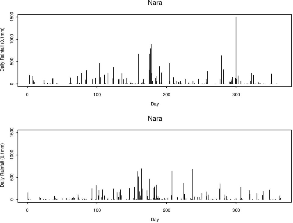
136 (median excess plot) u < x max { {(u, median 1 i nu x[i] u }) } : u < x max u u ẽ(v) = σ(2 ξ 1)/ξ + (2 ξ 1)v, ξ 0, σ log 2, ξ = 0.

137 ξ σ u < x max {x [i] u} n u i=1 GP(σ u, ξ) σ u ξ u (u, σ ) (u, ξ) σ = σ u ξu u σ ξ u Y v Y > v GP(σ + ξv, ξ) (v > 0), σ v = σ + ξv.

138 Pareto Hill ξ > 0 m x (1) x (2) x (m) {( ( ) ) } i log, log x (i), i = 1, 2,..., m m + 1 x (k+1) x (k+1) Hill (Hill, 1975) ξ H (k) = 1 k k i=1 ( log x (i) log x (k+1) ) k ξ H (k) k x (k+1)

139 GP(σ, ξ) GP y (1) y (2)... y (n) {( Ĥ(y (i) ), i n + 1 Ĥ(y (i) ) = 1 ( ) } : i = 1,..., n 1 + ξ y (i) σ ) 1/ ξ.

140 {( Ĥ 1 ( i n + 1 ), y (i) ) } : i = 1,..., n Ĥ 1 ( i n + 1 ) = σ ( n + 1 i n + 1 ) ξ 1 / ξ. { m (log m, x m ) } [ (m x m = u + σ ζ ]/ ) ξ u 1 ξ.

141 GP GP X 1, X 2,... t s(t) X t u s(t) X t > u s(t) GP(σ s(t), ξ s(t) ). u s(t) s(t) σ ξ s(t) s(t)

142 GP Y t GP(σ(t), ξ(t)) Y 0 = 1 { ξ(t) log 1 + ξ(t) Y } t σ(t) GP(1, 0) : P (Y 0 y) = H 0 (z) = 1 exp( y), 0 < y <. y t1, y t2,..., y tk σ(t) ξ(t) β ỹ tk = 1 ξ(t) log { 1 + ξ(t) y t i σ(t) }, i = 1, 2,..., k

143 ỹ (1) ỹ (2) ỹ (k) {( 1 exp( ỹ (i) ), {( ( log 1 i k + 1 i k + 1 ) ), ỹ (i) ) } : i = 1,..., k } : i = 1,..., k

144 Anderson & Coles (2002) Beirlant et al. (2004) clean bearing steel 5µm Diameter

145 Mean Excess u

146 Modified Scale Threshold Shape Threshold σ ξ

147 GP 5 ξ = (0.0914), σ = 1.68 (0.220) PP QQ

148 Probability Plot Quantile Plot Empirical Empirical Model Model

149 0.1mm GP

150 Daily Rainfall Nara (0.1mm)

151 Mean Excess u

152 Modified Scale Threshold Shape Threshold σ ξ

153 u 300 Coles (2001) u σ ξ u = (σ, ξ) σ = (12.541), ξ = (0.0512). GP

154 Probability Plot Quantile Plot Empirical Empirical Model Return Level Plot Model Density Plot Return level f(x) Return period (years) x

155 ξ ξ ξ 95% [ 0.020, 0.183] 100 ẑ 1/100 = % [1567, 2633]

156 Profile Log-likelihood Shape Parameter ξ ξ = (0.0512) 95% [ 0.020, 0.183]

157 Profile Log-likelihood Return Level z 1/100 ẑ 1/100 = % [1567, 2633]

158 GP GP(σ, ξ) ? GP

159 DailyRainfall Nara DailyRainfall Nara (0.1mm) 1961 ( 1962 (

160 σ = (13.901), ξ = (0.0540). ξ z 1/100 ξ z 1/100 95% [ 0.032, 0.182] [1559, 2649] declustering Coles (2001) 5.3.2

161 Probability Plot Quantile Plot Empirical Empirical Model Return Level Plot Model Density Plot Return level f(x) Return period (years) x

162 Profile Log-likelihood Shape Parameter ξ ξ = (0.0540) 95% [ 0.032, 0.182]. [ 0.020, 0.183]

163 Profile Log-likelihood Return Level z 1/100 z 1/100 95% [1559, 2649] [1567, 2633]

164 (PP) u (0, 1) (u, ) N n Poisson N A = (0, 1) (u, ) { (t1, x 1 ),..., (t N(A), x N(A) ) } A N n N A = [0, 1] (u, ) Λ(A) = [ 1 + ξ ( z µ σ )] 1/ξ

165 n y L A (µ, σ, ξ; x 1,..., x n ) = exp { Λ(A) } N(A) i=1 λ(t i, x i ) exp { n y [ 1 + ξ ( u µ σ )] 1/ξ } N(A) i=1 1 σ [ 1 + ξ ( xi µ σ )] 1/ξ 1 ( µ, σ, ξ)

166 PP 0.1 C PP Coles (2001) u(t) = sin(2π(t 110)/365.25)

167 Daily Maximum Temperature Kyoto (0.1 C)

168 Coles (2001) µ(t) = β 0 + β 1 sin(2πt/365.25) + β 2 cos(2πt/365.25), log σ(t) = β 3 + β 4 sin(2πt/365.25) + β 5 cos(2πt/365.25). ξ Coles S-Plus β 0 = (1.100), β 1 = (1.377), β 2 = (2.033), β 3 = (0.1335), β 4 = (0.0465), β 5 = (0.0684), ξ = (0.0473)

169 Residual Probability Plot Residual quantile Plot (Exptl. Scale) Empirical Empirical Model Model

170

1 Tokyo Daily Rainfall (mm) Days (mm)

1 Tokyo Daily Rainfall (mm) Days (mm) ( ) r-taka@maritime.kobe-u.ac.jp 1 Tokyo Daily Rainfall (mm) 0 100 200 300 0 10000 20000 30000 40000 50000 Days (mm) 1876 1 1 2013 12 31 Tokyo, 1876 Daily Rainfall (mm) 0 50 100 150 0 100 200 300 Tokyo,